4.4 Achievable Kernel Bandwidth

Published on 2018-05-13 | Category: CUDA, Freshman | Comments: 0 | Views:

Abstract: This article uses matrix transposition as an example to adjust and optimize kernel functions to achieve optimal memory bandwidth.

Keywords: Bandwidth, Throughput, Matrix Transposition

Achievable Kernel Bandwidth

In the previous chapter, we studied how to achieve maximum SM utilization by adjusting thread grid structure and kernel functions. Today we will study how to achieve maximum memory bandwidth utilization.

Let me mention that old example again. Honestly, it is very vivid and useful. Remembering this example essentially tells you where to start with CUDA optimization:

**A main road (memory read bus) connects the factory workshop (GPU) to the material warehouse (global memory). The workshop has many work groups (SMs), and the warehouse has many small storage rooms (memory partitions). Work groups produce the same products simultaneously without interfering with each other (parallelism). We have trucks driving from the warehouse to the factory. When to depart and what to transport is dictated by the work groups via remote phone calls (memory requests). Before departure, when loading materials from the warehouse, the trucks must also follow the warehouse manager's allocation, because the same storage room may only allow one truck at a time (memory block access blocking). These trucks then drive one-way to the factory -- this is where traffic management comes in. If our road is one-way (from warehouse to factory) with 8 lanes and can pass 16 trucks per second, we call this metric bandwidth. We also have a road for transporting finished products to the finished goods warehouse. This road is separate from the raw materials warehouse, and like the road from the materials warehouse to the factory, it has its own width and is one-way. If this road is blocked, just like the road from the warehouse to the factory, the factory must stop and wait.

The ideal state is: the road is full of trucks, all driving at high speed, and all workers in the factory are working at full capacity with no waiting. This is the ultimate goal of optimization. If this goal is achieved and you want to further improve efficiency, you can only optimize your processes (algorithms).**

The above is a rough description of the GPU working process. The example is quite fitting but somewhat loosely described -- reading it a couple more times should yield some insights.

Memory latency is a critical factor affecting kernel functions. Memory latency is the total time from when you initiate a memory request to when the data enters the SM's registers.

Memory bandwidth is the speed at which the SM accesses memory, measured in bytes transferred per unit time.

In the previous section, we used two methods to improve kernel performance:

• Maximize the number of warps to hide memory latency, maintaining more executing memory accesses for better bus utilization
• Improve bandwidth efficiency through proper alignment and coalesced access

However, the current kernel's memory access method is inherently problematic. The above optimizations are like optimizing the aerodynamics of a tractor -- a drop in the bucket.

What we want to do in this article is examine the problem corresponding to this kernel, determine its peak efficiency, and then optimize. We will use matrix transposition as a study case to see how to redesign a seemingly unoptimizable kernel to achieve better performance.

Memory Bandwidth

Most kernels are bandwidth-sensitive, meaning workers are extremely efficient but raw materials arrive slowly, limiting production speed. Depending on how data is arranged in memory and how warps access it, bandwidth is significantly affected. There are generally two types of bandwidth:

• Theoretical Bandwidth
• Effective Bandwidth

Theoretical bandwidth is the absolute maximum of the hardware design. For example, the Fermi M2090 without ECC has a theoretical peak of 117.6 GB/s.

Effective bandwidth is the bandwidth actually achieved by the kernel function -- a measured bandwidth. It can be calculated with the following formula: Effective Bandwidth = (Bytes Read + Bytes Written) x 10^-9 / Execution Time ... (1)

Note the difference between throughput and bandwidth. Throughput measures computational core efficiency and is measured in GFLOPS (Giga Floating-point Operations Per Second). Effective throughput depends not only on effective bandwidth but also on bandwidth utilization and other factors. Of course, the most important factor is the device's computational cores.

There is also a concept of memory throughput, which measures the total amount of memory access per unit time, in GB/s. A higher value means more data is read, but this data is not necessarily useful.

Next, we study how to adjust kernel functions to improve effective bandwidth.

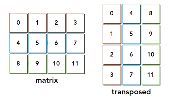
Matrix Transposition Problem

Matrix transposition swaps the row and column coordinates of a matrix. We study 2D matrices in this article, with the transposition result as follows:

Serial programming makes this easy to implement:

void transformMatrix2D_CPU(float * MatA, float * MatB, int nx, int ny)
{
    for(int j = 0; j < ny; j++)
    {
        for(int i = 0; i < nx; i++)
        {
            MatB[i*nx+j] = MatA[j*nx+i];
        }
    }
}

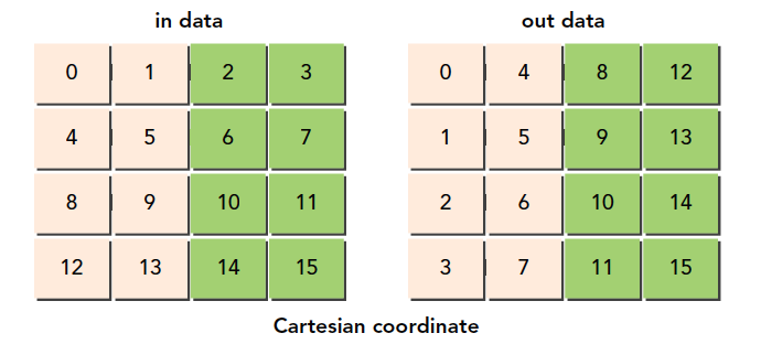
This code should be easy to understand -- it is a serial solution. What must be noted is that all our data, whether structures, arrays, or multi-dimensional arrays, is laid out one-dimensionally at the hardware memory level. So we also use a one-dimensional array as input and output. From a realistic perspective, the data in memory looks like this:

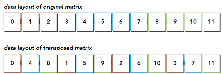
From this diagram, we can conclude that the transposition operation:

• Read: The original matrix is read row by row, and the requested memory is contiguous, allowing coalesced access
• Write: Writing to the transposed matrix's columns results in interleaved access

Pay attention to the colors in the diagram. During the read process, the same color can be seen as coalesced reads. But after transposition, the write process is interleaved.

Interleaved access is the primary culprit for degrading memory access. However, for matrix transposition itself, this is unavoidable. But under this unavoidable interleaved access, how to improve efficiency becomes an interesting topic.

All our subsequent methods will have both row-read and column-read versions to compare efficiency, to see whether interleaved reads or interleaved writes have the advantage.

Based on our previous analysis, if we read using the following two methods:

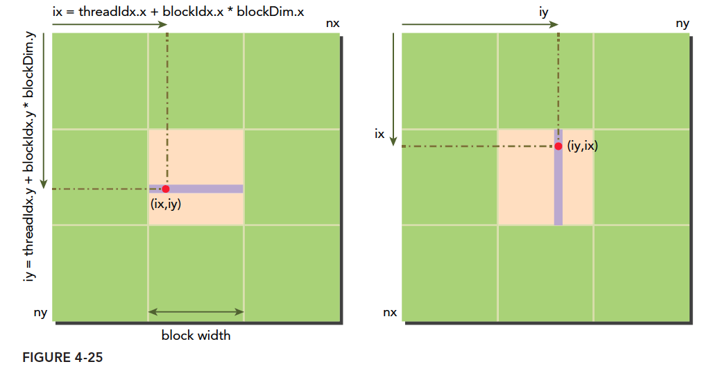
The initial thought is definitely: coalesced reads as in Figure 1 are more efficient, because writes don't go through L1 cache, so for programs with L1, coalesced reads should be more efficient. If you think this, congratulations -- you are wrong (I thought so too at the time).

We need to add some information about L1 cache's role. Earlier when we discussed coalescing, the first impression might be that L1 is a buffer for data coming from global memory. But we overlooked something: when a load request is initiated, the L1 cache is first checked for the data. If present, it is a hit -- this operates the same as CPU caches. If it hits, there is no need to read from global memory. In the above example, although reading by column is not coalesced, the data loaded via L1 will be used later. We must note that although L1 reads 128 bytes at a time with only one unit being useful, the rest is not immediately overwritten. The granularity is 128 bytes, but L1 is several KB or larger, so the data is unlikely to be replaced. So when reading by column, although only one element is used for the first row, when reading the next column, ideally all needed elements are already in L1. At this point, data is read directly from the cache -- excellent!

Setting Upper and Lower Bounds for the Transposition Kernel

Before optimization, we need to set a target -- what is the theoretical limit? For example, if the theoretical limit is 10 and we have already spent a day optimizing to 9.8, there is no need to spend another 10 days optimizing to 9.9 because it is already very close to the limit. Without knowing the limit, time is wasted in asymptotic improvement.

The bottleneck in our example is interleaved access, so we assume no interleaved access and all interleaved access to give upper and lower bounds:

• Row-read, row-store to copy the matrix (upper bound)
• Column-read, column-store to copy the matrix (lower bound)

__global__ void copyRow(float * MatA, float * MatB, int nx, int ny)
{
    int ix = threadIdx.x + blockDim.x * blockIdx.x;
    int iy = threadIdx.y + blockDim.y * blockIdx.y;
    int idx = ix + iy * nx;
    if (ix < nx && iy < ny)
    {
        MatB[idx] = MatA[idx];
    }
}

__global__ void copyCol(float * MatA, float * MatB, int nx, int ny)
{
    int ix = threadIdx.x + blockDim.x * blockIdx.x;
    int iy = threadIdx.y + blockDim.y * blockIdx.y;
    int idx = ix * ny + iy;
    if (ix < nx && iy < ny)
    {
        MatB[idx] = MatA[idx];
    }
}

We compile with command line, enabling L1 cache:

nvcc -O3 -arch=sm_35 -Xptxas -dlcm=ca -I ../include/ transform_matrix2D.cu -o transform_matrix2D

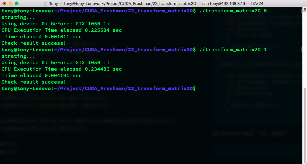
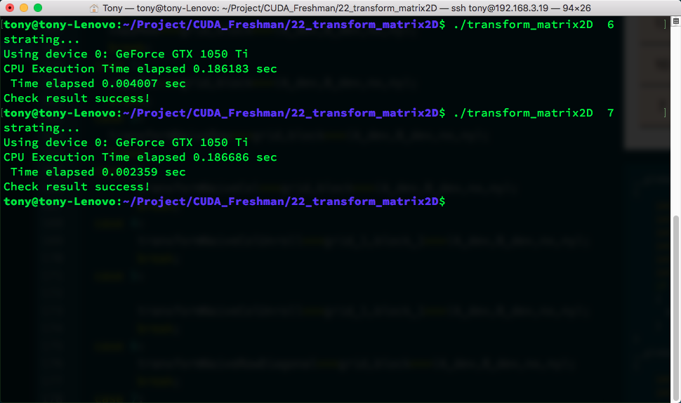
Results:

Kernel	Trial 1	Trial 2	Trial 3	Average
Upper Bound	0.001611	0.001614	0.001606	0.001610
Lower Bound	0.004191	0.004210	0.004205	0.004202

These times are averages from three tests. We can be fairly confident that at the current data scale, the upper bound is 0.001610s and the lower bound is 0.004202s. It is impossible to exceed the upper bound, and if you can break below the lower bound, that would be impressive!

Additionally, the main function used throughout the article is listed here only once. The complete code repository is at https://github.com/Tony-Tan/CUDA_Freshman

int main(int argc, char** argv)
{
    printf("starting...\n");
    initDevice(0);
    int nx = 1 << 12;
    int ny = 1 << 12;
    int nxy = nx * ny;
    int nBytes = nxy * sizeof(float);
    int transform_kernel = 0;
    if(argc >= 2)
        transform_kernel = atoi(argv[1]);
    
    //Malloc
    float* A_host = (float*)malloc(nBytes);
    float* B_host = (float*)malloc(nBytes);
    initialData(A_host, nxy);

    //cudaMalloc
    float *A_dev = NULL;
    float *B_dev = NULL;
    CHECK(cudaMalloc((void**)&A_dev, nBytes));
    CHECK(cudaMalloc((void**)&B_dev, nBytes));

    CHECK(cudaMemcpy(A_dev, A_host, nBytes, cudaMemcpyHostToDevice));
    CHECK(cudaMemset(B_dev, 0, nBytes));

    int dimx = 32;
    int dimy = 32;

    // cpu compute
    double iStart = cpuSecond();
    transformMatrix2D_CPU(A_host, B_host, nx, ny);
    double iElaps = cpuSecond() - iStart;
    printf("CPU Execution Time elapsed %f sec\n", iElaps);

    // 2d block and 2d grid
    dim3 block(dimx, dimy);
    dim3 grid((nx-1)/block.x+1, (ny-1)/block.y+1);
    dim3 block_1(dimx, dimy);
    dim3 grid_1((nx-1)/(block_1.x*4)+1, (ny-1)/block_1.y+1);
    
    iStart = cpuSecond();
    switch(transform_kernel)
    {
    case 0:
        copyRow<<<grid, block>>>(A_dev, B_dev, nx, ny);
        break;
    case 1:
        copyCol<<<grid, block>>>(A_dev, B_dev, nx, ny);
        break;
    case 2:
        transformNaiveRow<<<grid, block>>>(A_dev, B_dev, nx, ny);
        break;
    case 3:
        transformNaiveCol<<<grid, block>>>(A_dev, B_dev, nx, ny);
        break;
    case 4:
        transformNaiveColUnroll<<<grid_1, block_1>>>(A_dev, B_dev, nx, ny);
        break;
    case 5:
        transformNaiveColUnroll<<<grid_1, block_1>>>(A_dev, B_dev, nx, ny);
        break;
    case 6:
        transformNaiveRowDiagonal<<<grid, block>>>(A_dev, B_dev, nx, ny);
        break;
    case 7:
        transformNaiveColDiagonal<<<grid, block>>>(A_dev, B_dev, nx, ny);
        break;
    default:
        break;
    }
    CHECK(cudaDeviceSynchronize());
    iElaps = cpuSecond() - iStart;
    printf(" Time elapsed %f sec\n", iElaps);
    CHECK(cudaMemcpy(B_host, B_dev, nBytes, cudaMemcpyDeviceToHost));
    checkResult(B_host, B_host, nxy);

    cudaFree(A_dev);
    cudaFree(B_dev);
    free(A_host);
    free(B_host);
    cudaDeviceReset();
    return 0;
}

The switch part could be written with function pointers, but it does not matter much (the original was likely written with function pointers).

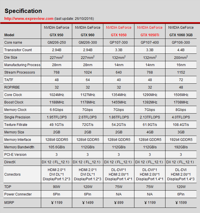
My laptop has a 1050Ti GPU. This table is likely the desktop version of the 1050Ti's specifications, showing a theoretical bandwidth of 112 GB/s:

Using formula (1) to calculate the bandwidth for both limits: copyRow = (1 x 2^12 + 12 x 4 x 2 x 10^-9) / 0.001610 = 0.134217728 / 0.001610 = 83.3650 GB/s

copyCol = (1 x 2^12 + 12 x 4 x 2 x 10^-9) / 0.004202 = 0.134217728 / 0.004202 = 31.9414 GB/s

Naive Transposition: Row Read vs Column Read

Next, let's look at the two most naive transposition methods, without any optimization -- the solutions we think of instantly:

__global__ void transformNaiveRow(float * MatA, float * MatB, int nx, int ny)
{
    int ix = threadIdx.x + blockDim.x * blockIdx.x;
    int iy = threadIdx.y + blockDim.y * blockIdx.y;
    int idx_row = ix + iy * nx;
    int idx_col = ix * ny + iy;
    if (ix < nx && iy < ny)
    {
        MatB[idx_col] = MatA[idx_row];
    }
}

__global__ void transformNaiveCol(float * MatA, float * MatB, int nx, int ny)
{
    int ix = threadIdx.x + blockDim.x * blockIdx.x;
    int iy = threadIdx.y + blockDim.y * blockIdx.y;
    int idx_row = ix + iy * nx;
    int idx_col = ix * ny + iy;
    if (ix < nx && iy < ny)
    {
        MatB[idx_row] = MatA[idx_col];
    }
}

Execution time:

Kernel	Trial 1	Trial 2	Trial 3	Average
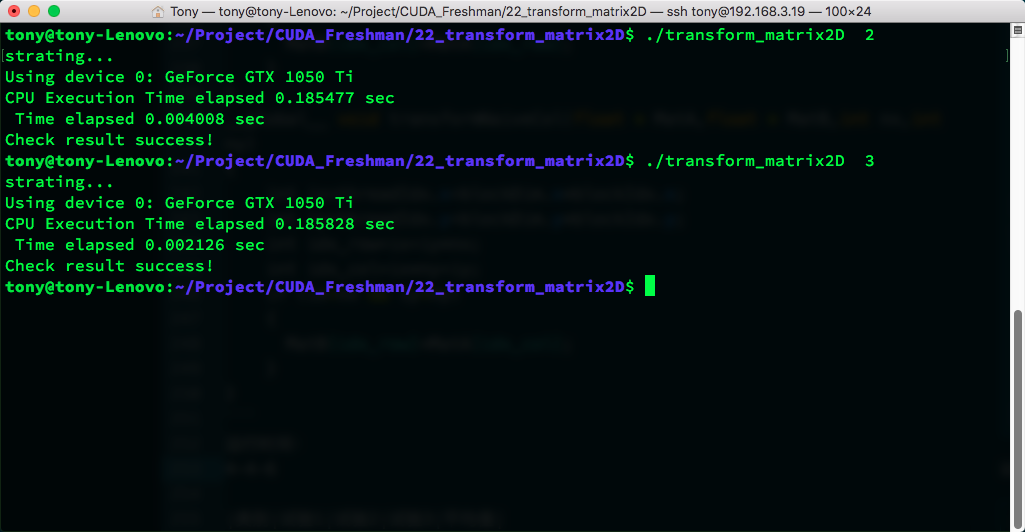
transformNaiveRow	0.004008	0.004005	0.004012	0.004008
transformNaiveCol	0.002126	0.002118	0.002124	0.002123

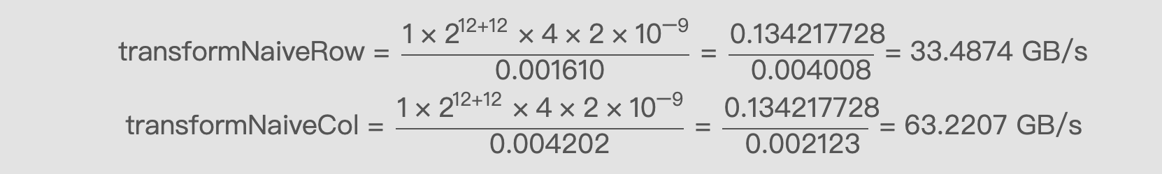
transformNaiveRow = 0.134217728 / 0.004008 = 33.4874 GB/s

transformNaiveCol = 0.134217728 / 0.002123 = 63.2207 GB/s

Reading by column is more effective, which is basically consistent with our analysis above.

Below is the L1 cache load/store throughput:

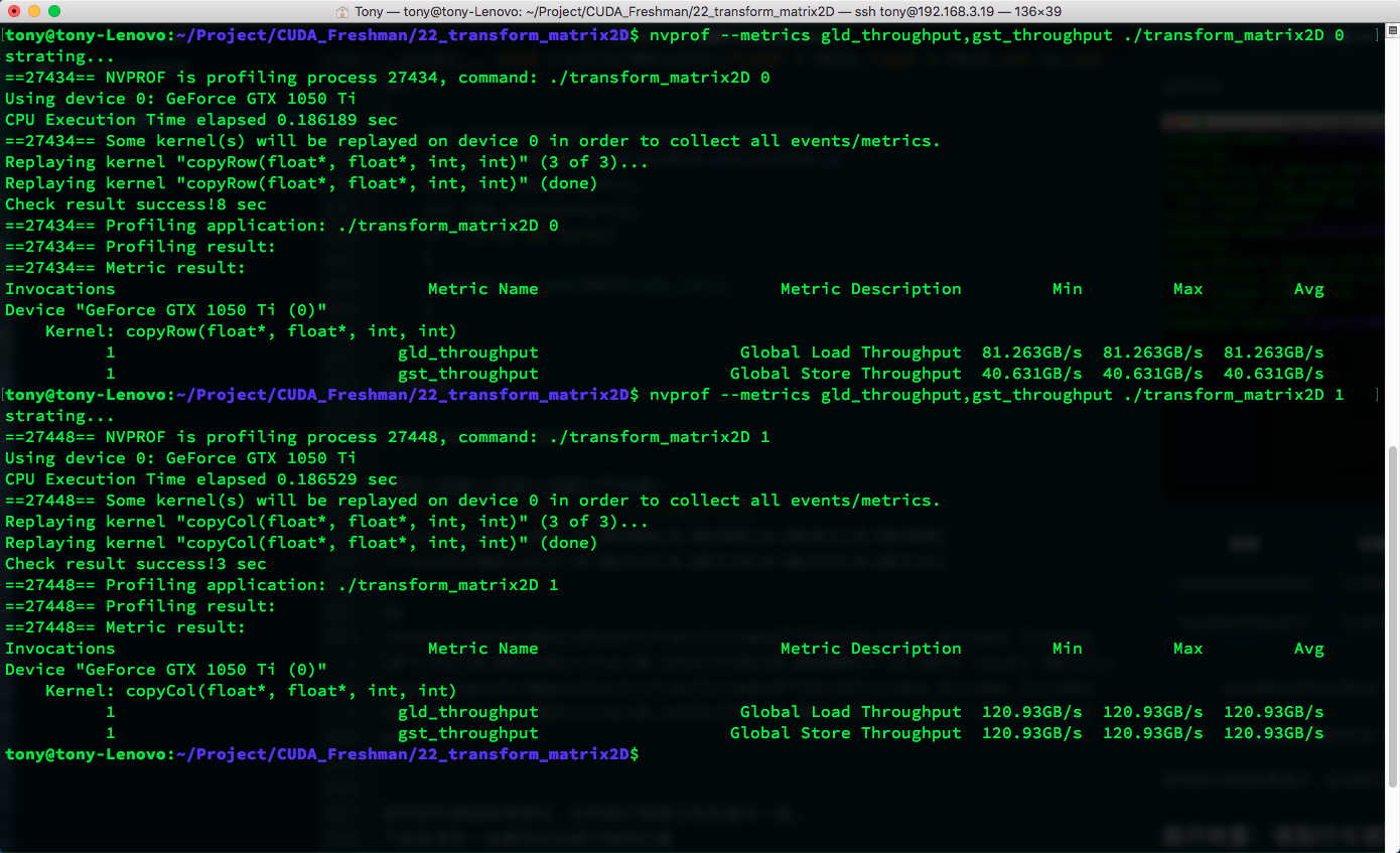
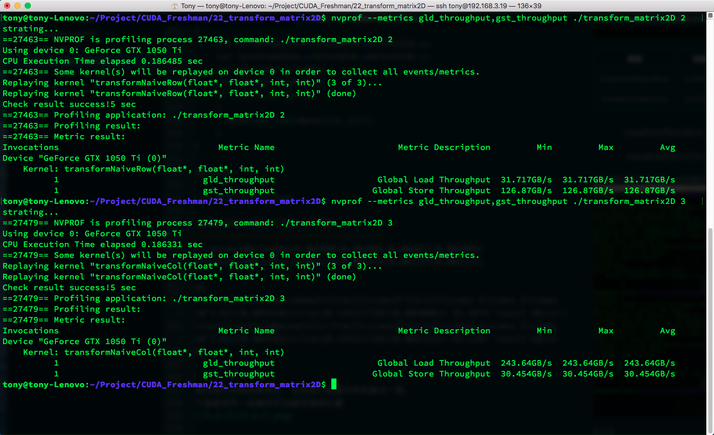
Kernel	Load Throughput	Store Throughput
copyRow	81.263	40.631
copyCol	120.93	120.93
transformNaiveRow	31.717	126.87
transformNaiveCol	243.64	30.454

The high throughput of column reads is due to the cache hits we discussed above. You can also see that throughput can exceed bandwidth because bandwidth measures the speed limit from global memory to SM, while throughput is the total data acquired by the SM divided by time. This data can come from L1 cache rather than making the long journey from main memory.

A question arises: although interleaved reads have higher cache hit rates, they do not seem to reduce the amount of data read from main memory. So why is there a speed improvement?

I believe it is the latency hiding aspect that makes interleaved reads more efficient. This is just my guess -- it needs verification later.

Unrolled Transposition: Row Read vs Column Read

The next technique is the old standby for effectively hiding latency -- starting with unrolling:

__global__ void transformNaiveRowUnroll(float * MatA, float * MatB, int nx, int ny)
{
    int ix = threadIdx.x + blockDim.x * blockIdx.x * 4;
    int iy = threadIdx.y + blockDim.y * blockIdx.y;
    int idx_row = ix + iy * nx;
    int idx_col = ix * ny + iy;
    if (ix < nx && iy < ny)
    {
        MatB[idx_col] = MatA[idx_row];
        MatB[idx_col + ny * 1 * blockDim.x] = MatA[idx_row + 1 * blockDim.x];
        MatB[idx_col + ny * 2 * blockDim.x] = MatA[idx_row + 2 * blockDim.x];
        MatB[idx_col + ny * 3 * blockDim.x] = MatA[idx_row + 3 * blockDim.x];
    }
}

__global__ void transformNaiveColUnroll(float * MatA, float * MatB, int nx, int ny)
{
    int ix = threadIdx.x + blockDim.x * blockIdx.x * 4;
    int iy = threadIdx.y + blockDim.y * blockIdx.y;
    int idx_row = ix + iy * nx;
    int idx_col = ix * ny + iy;
    if (ix < nx && iy < ny)
    {
        MatB[idx_row] = MatA[idx_col];
        MatB[idx_row + 1 * blockDim.x] = MatA[idx_col + ny * 1 * blockDim.x];
        MatB[idx_row + 2 * blockDim.x] = MatA[idx_col + ny * 2 * blockDim.x];
        MatB[idx_row + 3 * blockDim.x] = MatA[idx_col + ny * 3 * blockDim.x];
    }
}

Results:

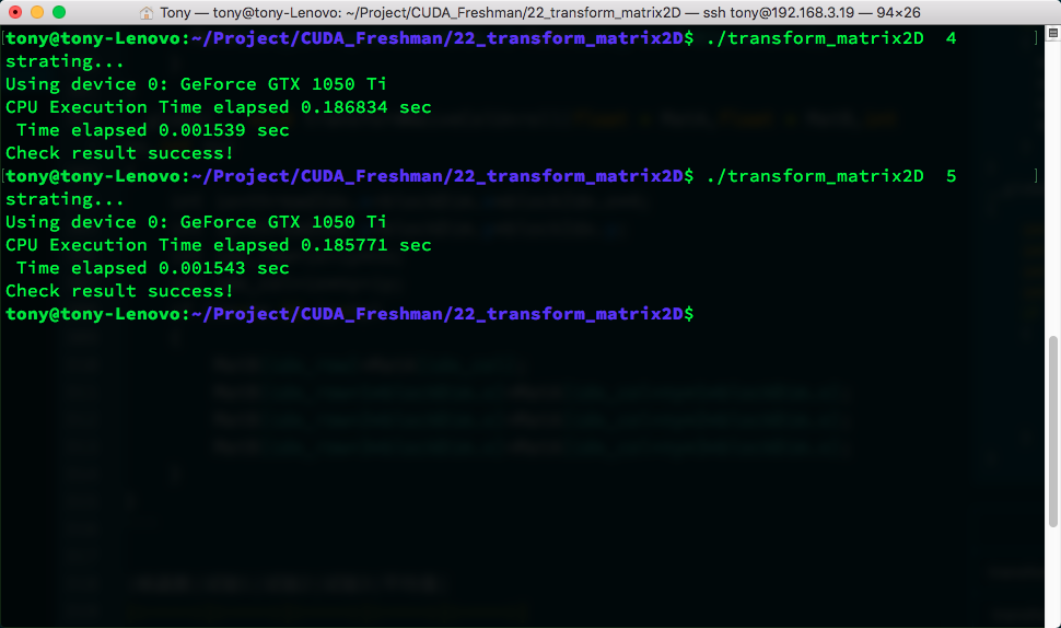
Kernel	Trial 1	Trial 2	Trial 3	Average
transformNaiveRowUnroll	0.001544	0.001550	0.001541	0.001545
transformNaiveColUnroll	0.001545	0.001539	0.001546	0.001543

An interesting phenomenon appeared here -- we broke through the upper bound. The upper bound was row-coalesced read and row-coalesced store with no interleaving. This ideal situation cannot happen in transposition, so we call it the upper bound. Yet our unrolled interleaved access achieved speeds faster than the upper bound. So I conclude that if the upper bound were also unrolled, it would definitely be even faster. But we still call this the upper bound here, even though it is not the true upper bound.

To know the true upper bound, you need to calculate the theoretical hardware upper bound. The measured upper bound may not be accurate.

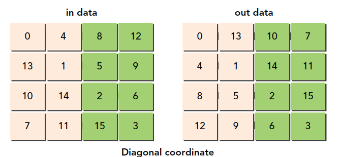
Diagonal Transposition: Row Read vs Column Read

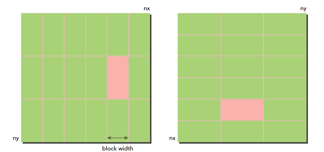
Next, we use a new trick derived from DRAM characteristics. Remember our example's description of the material warehouse with many small storage rooms? These rooms may only allow one truck at a time. In DRAM, memory is partitioned. If too many accesses go to the same partition, queuing occurs -- causing waits. To avoid this, we should spread accesses evenly across a range of DRAM. DRAM partitions are every 256 bytes, so we should stagger accesses to the same partition by adjusting block IDs. You might wonder: we don't know the block execution order, so how do we adjust? There is no official explanation for this. My understanding is that hardware must execute thread blocks following some rule. Executing in order 1-2-3 is probably better than random execution, because random execution requires an additional step to generate random order -- which is unnecessary. The reason we say block execution order is undefined is to prevent people from assuming a fixed order, when in practice certain factors may cause the order to vary. But this is definitely not intentionally designed by hardware.

The purpose of our diagonal transposition is to spread DRAM accesses more evenly, avoiding concentration in a single partition. The method is to scramble thread blocks, since consecutive thread blocks may access nearby DRAM addresses.

Our approach uses a function f(x,y)=(m,n), a one-to-one mapping that scrambles the original Cartesian coordinates.

Note that all these thread block orderings are on the programming model level and have nothing to do with hardware. These are logical concepts. Which thread block ID corresponds to which thread block is also something we define ourselves.

Honestly, this code is somewhat difficult to understand. But you don't need to memorize this technique -- programmers don't memorize code, and even the learning process doesn't require memorization. What we need to understand is the mapping between thread block IDs and thread blocks, and the mapping between new IDs and original IDs, and which blocks the new IDs correspond to.

Original thread block IDs:

Newly designed thread block IDs:

__global__ void transformNaiveRowDiagonal(float * MatA, float * MatB, int nx, int ny)
{
    int block_y = blockIdx.x;
    int block_x = (blockIdx.x + blockIdx.y) % gridDim.x;
    int ix = threadIdx.x + blockDim.x * block_x;
    int iy = threadIdx.y + blockDim.y * block_y;
    int idx_row = ix + iy * nx;
    int idx_col = ix * ny + iy;
    if (ix < nx && iy < ny)
    {
        MatB[idx_col] = MatA[idx_row];
    }
}

__global__ void transformNaiveColDiagonal(float * MatA, float * MatB, int nx, int ny)
{
    int block_y = blockIdx.x;
    int block_x = (blockIdx.x + blockIdx.y) % gridDim.x;
    int ix = threadIdx.x + blockDim.x * block_x;
    int iy = threadIdx.y + blockDim.y * block_y;
    int idx_row = ix + iy * nx;
    int idx_col = ix * ny + iy;
    if (ix < nx && iy < ny)
    {
        MatB[idx_row] = MatA[idx_col];
    }
}

This speed is not faster than the unrolled version, nor even as fast as the naive interleaved read. But the book says efficiency improved -- possibly due to CUDA version updates or other factors. However, the DRAM partition queuing phenomenon is worth noting.

Thin Blocks to Increase Parallelism

Next is the old trick of adjusting thread block sizes to see if anything changes. We use the naive column read as a baseline.

Block Size	Test 1	Test 2	Test 3	Average
(32,32)	0.002166	0.002122	0.002125	0.002138
(32,16)	0.001677	0.001696	0.001703	0.001692
(32,8)	0.001925	0.001929	0.001925	0.001926
(64,16)	0.002117	0.002146	0.002113	0.002125
(64,8)	0.001949	0.001945	0.001945	0.001946
(128,8)	0.002228	0.002230	0.002229	0.002229

These are simple experimental results. The (32, 16) configuration has the highest efficiency:

Summary

This article mainly explains the impact of memory bandwidth on efficiency and how to effectively break through memory access bottlenecks by adjusting read methods. This is a very important technique for optimizing CUDA programs.