3.3 Parallelism and Performance

Published 2018-04-15 | Category: CUDA, Freshman | Comments: 0 | Read count:

Abstract: This article mainly uses the nvprof tool to analyze kernel function execution efficiency (resource utilization).

Keywords: nvprof

Parallelism and Performance

Continuing with CUDA updates. I paused CUDA for a while to accelerate my probability theory studies. Starting today, I'm resuming updates for both CUDA and mathematical analysis. Writing a bit of rambling at the beginning of each article is like a diary. I used to admire people who kept diaries because I had no idea what to write about. But now I see that writing words to record yourself, first, lets you reflect on the present, and second, lets you check later whether you've actually made progress. These are all useful, so feel free to skip my rambling and go straight to the main content.

The main content of this article is to further understand the essential process of warp execution on hardware. Combined with the previous articles on the execution model, this article's content is relatively simple. By modifying kernel configurations, we observe kernel execution speed and analyze hardware utilization data to assess performance. Adjusting kernel configurations is a skill CUDA developers must master. This article only studies how kernel configuration affects efficiency (obtaining different execution efficiencies through grid and block configurations).

This entire article uses only the following kernel function:

__global__ void sumMatrix(float * MatA, float * MatB, float * MatC, int nx, int ny)
{
    int ix = threadIdx.x + blockDim.x * blockIdx.x;
    int iy = threadIdx.y + blockDim.y * blockIdx.y;
    int idx = ix + iy * ny;
    if (ix < nx && iy < ny)
    {
        MatC[idx] = MatA[idx] + MatB[idx];
    }
}

The simplest 2D matrix addition with no optimization whatsoever.

Complete code:

int main(int argc, char** argv)
{
    //printf("strating...\n");
    //initDevice(0);
    int nx = 1 << 13;
    int ny = 1 << 13;
    int nxy = nx * ny;
    int nBytes = nxy * sizeof(float);

    //Malloc
    float* A_host = (float*)malloc(nBytes);
    float* B_host = (float*)malloc(nBytes);
    float* C_host = (float*)malloc(nBytes);
    float* C_from_gpu = (float*)malloc(nBytes);
    initialData(A_host, nxy);
    initialData(B_host, nxy);

    //cudaMalloc
    float *A_dev = NULL;
    float *B_dev = NULL;
    float *C_dev = NULL;
    CHECK(cudaMalloc((void**)&A_dev, nBytes));
    CHECK(cudaMalloc((void**)&B_dev, nBytes));
    CHECK(cudaMalloc((void**)&C_dev, nBytes));

    CHECK(cudaMemcpy(A_dev, A_host, nBytes, cudaMemcpyHostToDevice));
    CHECK(cudaMemcpy(B_dev, B_host, nBytes, cudaMemcpyHostToDevice));

    int dimx = argc > 2 ? atoi(argv[1]) : 32;
    int dimy = argc > 2 ? atoi(argv[2]) : 32;

    double iStart, iElaps;

    // 2d block and 2d grid
    dim3 block(dimx, dimy);
    dim3 grid((nx-1)/block.x+1, (ny-1)/block.y+1);
    iStart = cpuSecond();
    sumMatrix<<<grid, block>>>(A_dev, B_dev, C_dev, nx, ny);
    CHECK(cudaDeviceSynchronize());
    iElaps = cpuSecond() - iStart;
    printf("GPU Execution configuration<<<(%d,%d),(%d,%d)|%f sec\n",
           grid.x, grid.y, block.x, block.y, iElaps);
    CHECK(cudaMemcpy(C_from_gpu, C_dev, nBytes, cudaMemcpyDeviceToHost));

    cudaFree(A_dev);
    cudaFree(B_dev);
    cudaFree(C_dev);
    free(A_host);
    free(B_host);
    free(C_host);
    free(C_from_gpu);
    cudaDeviceReset();
    return 0;
}

As you can see, we use two 8192x8192 matrices being added to test our efficiency.

Note the GPU memory here: one matrix is 2^13 x 2^13 x 2^2 = 2^28 bytes, which is 256MB. Three matrices total 768MB. Since our GPU memory is only 2GB, we can't do larger matrix computations (we can't use the 2^14 square matrices from the original text).

Detecting Active Warps with nvprof

For performance comparison, we need to control variables. The code above uses only two variables: the x and y sizes of the block. So, adjusting x and y produces different efficiencies. Let's look at the results first:

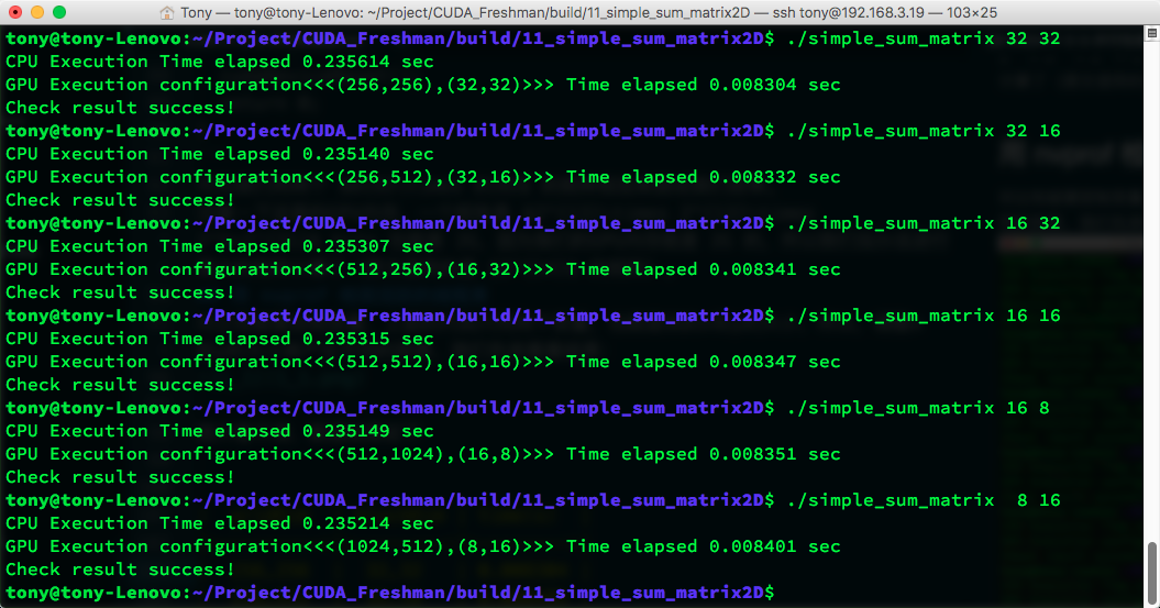
The image is hard to read. The data results are:

gridDim	blockDim	time(s)
256,256	32,32	0.008304
256,512	32,16	0.008332
512,256	16,32	0.008341
512,512	16,16	0.008347
512,1024	16,8	0.008351
1024,512	8,16	0.008401

When the block size exceeds hardware limits, it doesn't throw an error but returns error values -- worth noting.

Also, each machine will produce different results for this code, so analyze data according to your own hardware.

The M2070 from the book gives different results from ours. The M2070's (32,16) configuration is most efficient, while ours is (32,32). After all, the architecture is different, and different CUDA versions lead to significant differences in optimized machine code. So let's look at the active warp situation using:

nvprof --metrics achieved_occupancy ./simple_sum_matrix

Results:

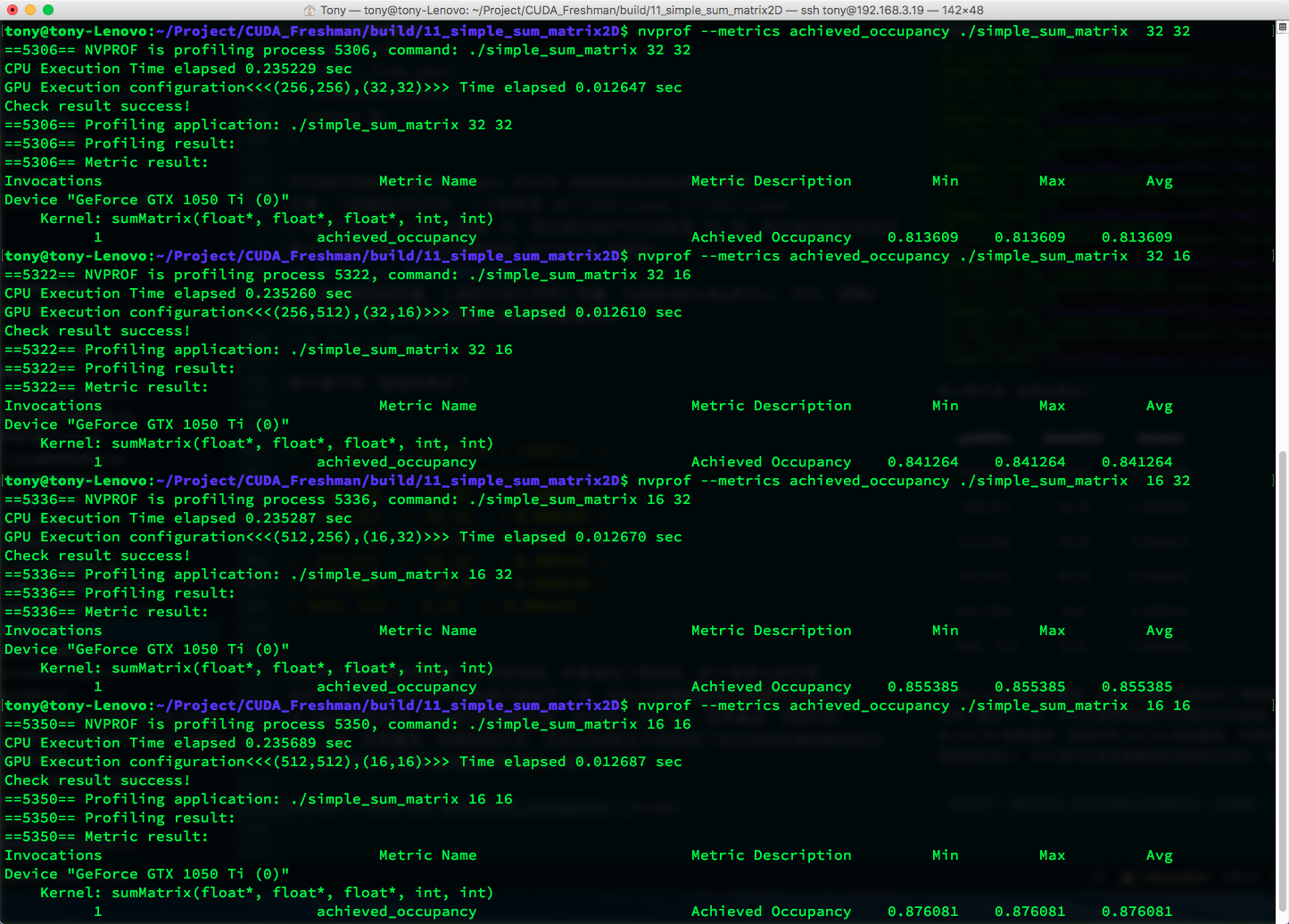
gridDim	blockDim	time(s)	Achieved Occupancy
256,256	32,32	0.008304	0.813609
256,512	32,16	0.008332	0.841264
512,256	16,32	0.008341	0.855385
512,512	16,16	0.008347	0.876081
512,1024	16,8	0.008351	0.875807
1024,512	8,16	0.008401	0.857242

Higher active warp ratio doesn't necessarily mean faster execution. In principle, higher utilization should mean higher efficiency, but other factors come into play.

The active warp ratio is defined as: the average number of active warps per cycle divided by the maximum warps supported by an SM.

Detecting Memory Operations with nvprof

Let's continue using nvprof to look at memory utilization.

First, use:

nvprof --metrics gld_throughput ./simple_sum_matrix

To look at the kernel's memory read efficiency:

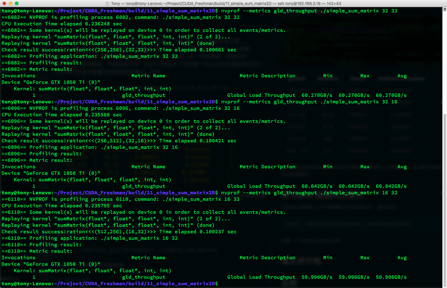
gridDim	blockDim	time(s)	Achieved Occupancy	GLD Throughput (GB/s)
256,256	32,32	0.008304	0.813609	60.270
256,512	32,16	0.008332	0.841264	60.042
512,256	16,32	0.008341	0.855385	59.996
512,512	16,16	0.008347	0.876081	59.967
512,1024	16,8	0.008351	0.875807	59.976
1024,512	8,16	0.008401	0.857242	59.440

Although the first configuration doesn't have the highest active warp ratio, it has the highest throughput. This shows that throughput and active warp ratio both affect final efficiency.

Next, let's look at global load efficiency. Global load efficiency is defined as: the ratio of requested global load throughput to required global load throughput (global load throughput). In other words, the degree to which the application's load operations utilize device memory bandwidth. Note the difference between throughput and global load efficiency -- we've already explained throughput in previous articles. If you've forgotten, go back and review.

nvprof --metrics gld_efficiency ./simple_sum_matrix

Results:

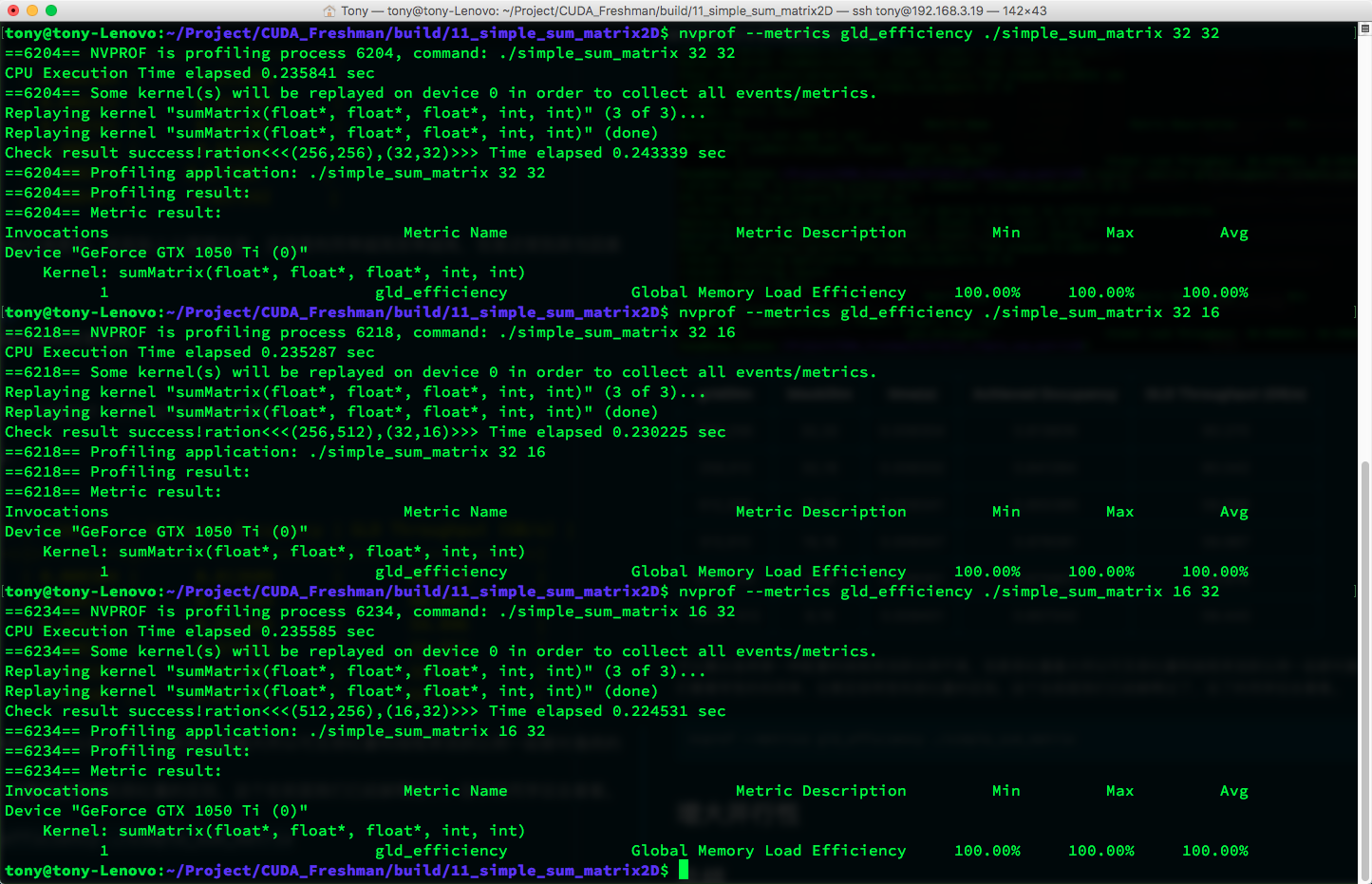
On the current machine, all utilization rates are 100%, meaning CUDA has optimized the kernel functions. On the M2070 with an older CUDA version, load efficiency wasn't this high. Effective load efficiency refers to how much of all memory requests (data currently being transferred on the bus) are actually used for computation.

The book says if the inner dimension of the thread block (blockDim.x) is too small -- less than a warp -- it affects load efficiency. But currently, this doesn't seem to be an issue.

As hardware advances, some previous issues may no longer be problems. Of course, for older devices, these tricks are still useful.

Increasing Parallelism

Let's see if the issue of "inner thread block dimension (blockDim.x) being too small" still affects current devices:

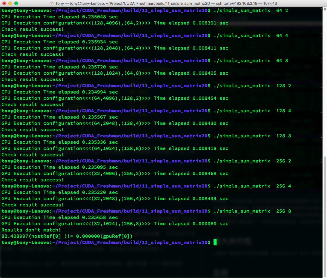
Data in tabular form:

gridDim	blockDim	time(s)
(128,4096)	(64,2)	0.008391
(128,2048)	(64,4)	0.008411
(128,1024)	(64,8)	0.008405
(64,4096)	(128,2)	0.008454
(64,2048)	(128,4)	0.008430
(64,1024)	(128,8)	0.008418
(32,4096)	(256,2)	0.008468
(32,2048)	(256,4)	0.008439
(32,1024)	(256,8)	fail

From this table, the fastest is still the first one -- the smallest block achieves the highest efficiency. This again differs from the book's results. I think the book's larger data volume may have influenced the results. With larger data volumes, the factors determining execution time may change. But some observations can be made:

• Although (64,4) and (128,2) have the same block size, they have different execution efficiencies, showing that the inner thread block dimension affects efficiency.
• The last block parameter is invalid.
• The first configuration is the fastest.

We adjust block sizes to increase parallelism, or rather, increase active warps. Let's look at warp occupancy:

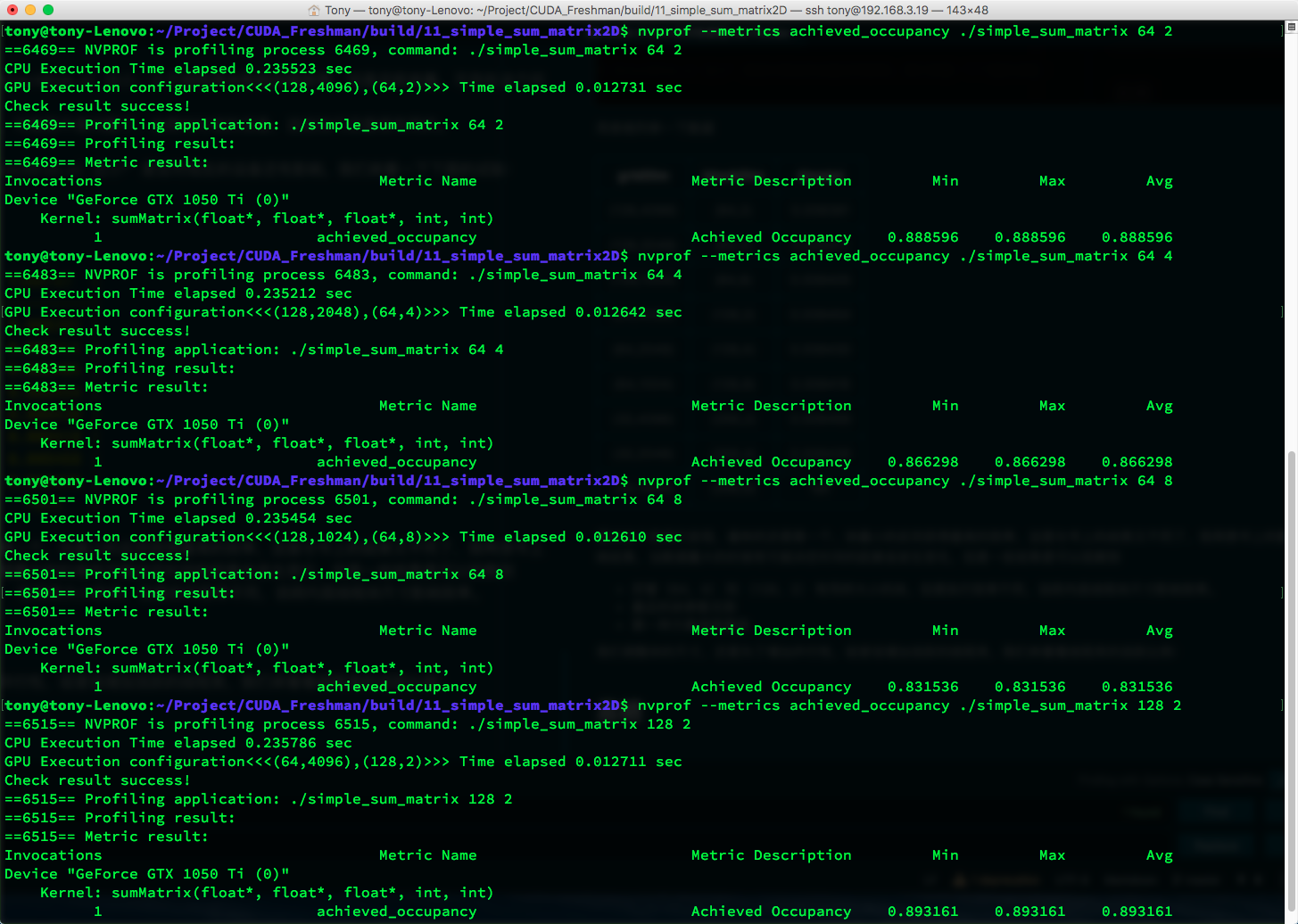
Data:

gridDim	blockDim	time(s)	Achieved Occupancy
(128,4096)	(64,2)	0.008391	0.888596
(128,2048)	(64,4)	0.008411	0.866298
(128,1024)	(64,8)	0.008405	0.831536
(64,4096)	(128,2)	0.008454	0.893161
(64,2048)	(128,4)	0.008430	0.862629
(64,1024)	(128,8)	0.008418	0.833540
(32,4096)	(256,2)	0.008468	0.859110
(32,2048)	(256,4)	0.008439	0.825036
(32,1024)	(256,8)	fail	Nan

The highest utilization doesn't yield the highest efficiency.

No single factor can directly determine final efficiency. Multiple factors work together to produce the final result -- a classic example of multiple causes yielding one effect. Therefore, when optimizing, we should first ensure the accuracy, objectivity, and stability of our timing measurements. Honestly, our timing method above isn't very stable. A more stable method would be to measure average time over multiple runs to reduce human error.

Summary

Metrics and performance:

• In most cases, a single metric cannot produce optimal performance
• What directly relates to overall performance is the kernel code itself (the kernel is the key)
• Metrics and performance require choosing a balance point
• Seek metric balance from different angles to maximize efficiency
• Grid and block sizes provide a good starting point for tuning performance

Starting from this point, we'll gradually dig into various metrics. In short, CUDA is all about efficiency, and studying these metrics is the fastest path to improving efficiency (though kernel algorithm improvements have even greater potential). Let me emphasize again: all data in this article applies only to my device. For any other device, these results would be completely different. Focus on learning these test metrics and their interrelationships.