3.4 Avoiding Branch Divergence
Abstract: Introduces the branch divergence problem in reduction operations.
Keywords: Reduction, Branch Divergence
Some results in this article differ from those in the reference book and require deeper technical investigation.
Avoiding Branch Divergence
This article introduces one of the most common and typical scenarios in parallel computing: branch divergence (an equivalent problem to warp divergence), along with reduction problems and their initial optimization.
Parallel Reduction Problem
In serial programming, one of the most common problems is reducing a large set of numbers to a single number through computation. For example, addition (computing the sum of a dataset) or multiplication. When such computations have the following characteristics, we can process them using parallel reduction:
- Associativity
- Commutativity
Addition and multiplication satisfy the commutative and associative laws. In our mathematical analysis series, we've already detailed the proofs of associativity and commutativity for addition and multiplication. So for all computations with these two properties, reduction-style computation can be used.
Why is it called "reduction"? Reduction is a common computation method (usable in both serial and parallel). When I first heard this name about two years ago, I was confused. Later I realized that reduction actually refers to recursively reducing the amount of data. Each iteration uses the same computation method (recursive property), ultimately going from a set of many numbers down to one number (reduction) -- which makes it very clear.
Reduction generally includes the following steps:
- Divide the input vector into smaller data blocks
- Use one thread to compute a partial sum of each data block
- Sum the partial sums of each data block to obtain the final result
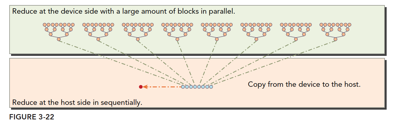
Data partitioning ensures we can use one thread block to process one data block. One thread processes a smaller block, so one thread block can process a larger block, and multiple blocks complete the entire dataset. Finally, sum the results from all thread blocks. This step is typically done on the CPU.
The most common reduction operation, addition, divides vector data into pairs, then uses different threads to compute each pair of elements. The results are used as input to form more pairs, iterated until a single element remains.
Common pairing methods include:
-
Adjacent Pairing: Elements are paired with their adjacent elements.
-
Interleaved Pairing: Elements are paired with elements at a certain distance.
The diagrams clearly illustrate both methods. Let's implement them in code.
First, the CPU version implementing interleaved pair reduction:
int recursiveReduce(int *data, int const size)
{
    // terminate check
    if (size == 1)
        return data[0];
    // renew the stride
    int const stride = size / 2;
    if (size % 2 == 1)
    {
        for (int i = 0; i < stride; i++)
        {
            data[i] += data[i + stride];
        }
        data[0] += data[size - 1];
    }
    else
    {
        for (int i = 0; i < stride; i++)
        {
            data[i] += data[i + stride];
        }
    }
    // call
    return recursiveReduce(data, stride);
}
This differs slightly from the book's code because the book's code doesn't account for array lengths that aren't powers of two. I added handling for the last unpaired element in odd-length arrays.
This addition operation can be changed to any computation satisfying associativity and commutativity, such as multiplication, finding the maximum, etc.
Now let's examine CUDA execution efficiency through different pairing methods and data organization.
Divergence in Parallel Reduction
Warp divergence clearly explains that wherever there's a conditional, branching occurs, such as if and for keywords.
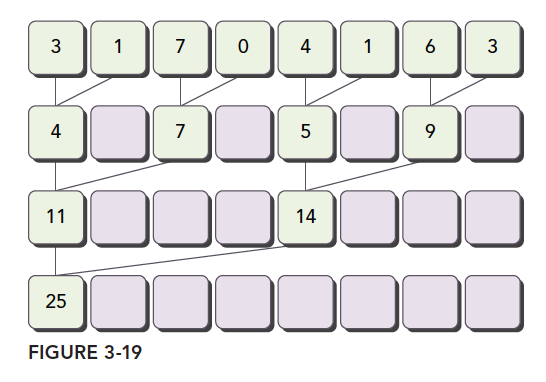
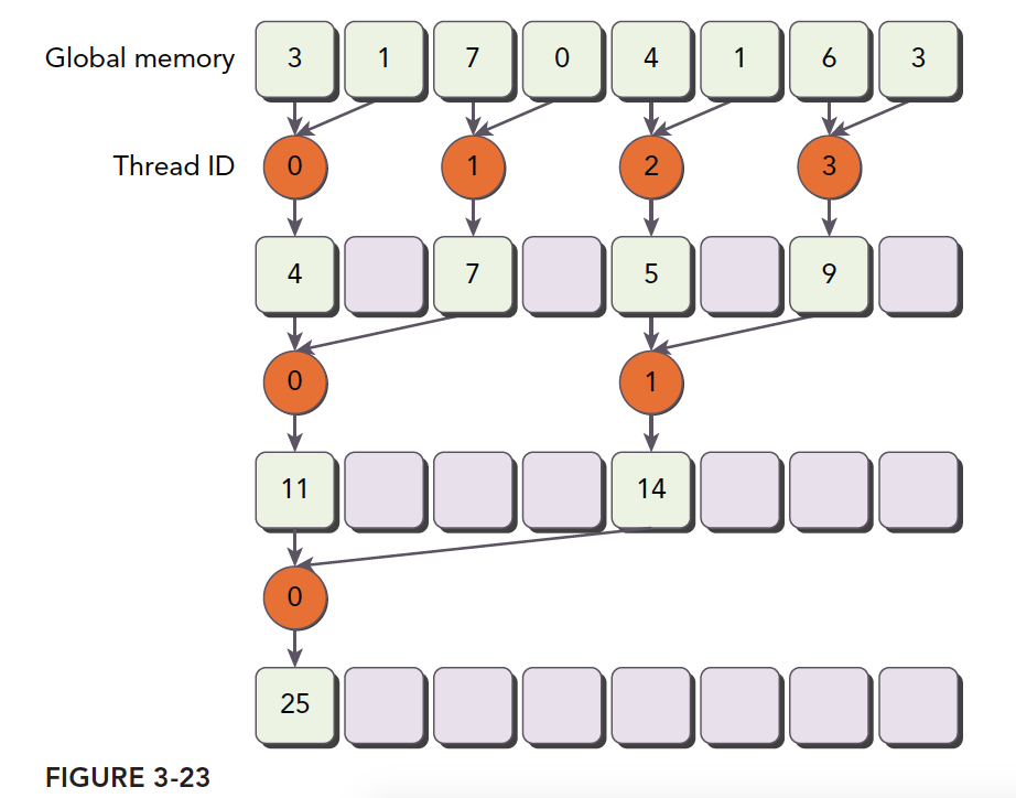
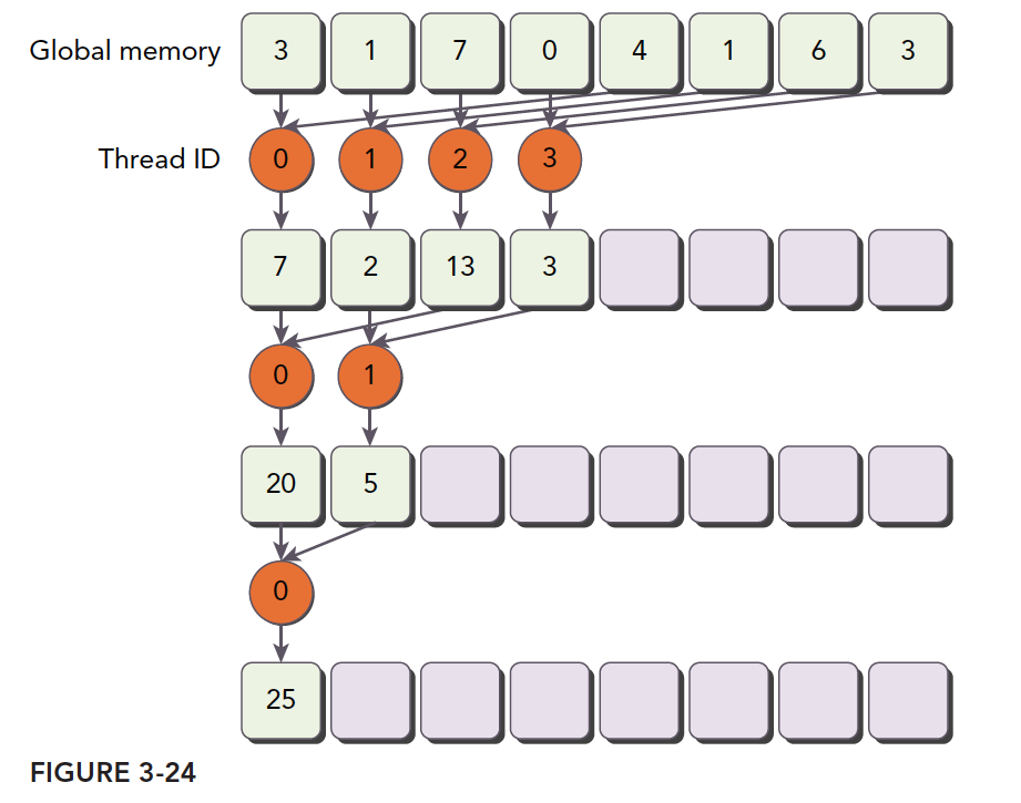
As shown below, our process description for adjacent element pairing in a kernel implementation:
(img)(https://tony4ai-1251394096.cos.ap-hongkong.myqcloud.com/blog_images/3_21.png)
Based on the previous section:
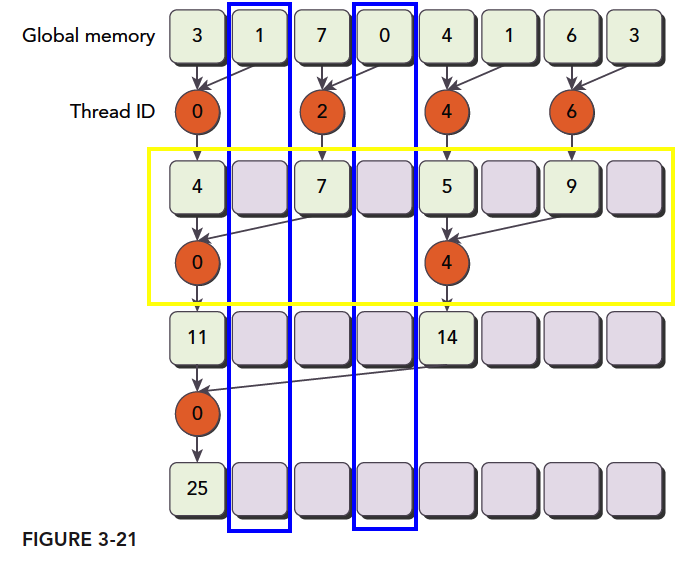
Step 1: Partition the array into blocks, each containing only partial data as shown above (the figure shows fewer data items, but we assume a block only has this many). We assume this is the complete data for a thread block.
Step 2: What each thread does. The orange circles represent each thread's operations. Thread threadIdx.x=0 performs three calculations. Odd-numbered threads are just along for the ride, never doing any computation. But as explained in 3.2, these threads, while doing nothing, cannot execute other instructions. Thread 4 does two steps, and threads 2 and 6 do only one step.
Step 3: Sum all block results to get the final result.
This computation partitioning is the simplest parallel reduction algorithm, completely following the three-step pattern we mentioned above.
Notably, each time we perform a round of computation (yellow box -- these operations happen simultaneously and in parallel), some global memory must be modified. But only part of it is replaced. The unreplaced portions won't be used later. As marked in the blue box, that memory is read once and then completely abandoned.
Now let's look at our kernel code:
__global__ void reduceNeighbored(int * g_idata, int * g_odata, unsigned int n)
{
    //set thread ID
    unsigned int tid = threadIdx.x;
    //boundary check
    if (tid >= n) return;
    //convert global data pointer to the
    int *idata = g_idata + blockIdx.x * blockDim.x;
    //in-place reduction in global memory
    for (int stride = 1; stride < blockDim.x; stride *= 2)
    {
        if ((tid % (2 * stride)) == 0)
        {
            idata[tid] += idata[tid + stride];
        }
        //synchronize within block
        __syncthreads();
    }
    //write result for this block to global mem
    if (tid == 0)
        g_odata[blockIdx.x] = idata[0];
}
The only thing to note here is the synchronization instruction:
__syncthreads();
The reason can still be seen in the diagram. Each round of our operations is parallel, but we can't guarantee all threads finish simultaneously. So we need to wait -- fast threads wait for slow ones. This avoids thread contention within a block for memory.
The distance between the two operated objects is called the stride, which is the variable stride.
The complete execution logic is shown below:
Note the boundary between host and device, and note the data partitioning on the device.
Complete executable code on Github: https://github.com/Tony-Tan/CUDA_Freshman
I'll paste the main function here, but note it includes the later kernel function execution parts. To run it, go clone it from github and give it a star while you're at it:
int main(int argc, char** argv)
{
    .........
    int size = 1 << 24;

    .........
    dim3 block(blocksize, 1);
    dim3 grid((size - 1) / block.x + 1, 1);

    .........

    //cpu reduction
    int cpu_sum = 0;
    iStart = cpuSecond();

    for (int i = 0; i < size; i++)
        cpu_sum += tmp[i];
    printf("cpu sum:%d \n", cpu_sum);
    iElaps = cpuSecond() - iStart;
    printf("cpu reduce                 elapsed %lf ms cpu_sum: %d\n", iElaps, cpu_sum);

    //kernel 1:reduceNeighbored
    CHECK(cudaMemcpy(idata_dev, idata_host, bytes, cudaMemcpyHostToDevice));
    CHECK(cudaDeviceSynchronize());
    iStart = cpuSecond();
    warmup <<<grid, block >>>(idata_dev, odata_dev, size);
    cudaDeviceSynchronize();
    iElaps = cpuSecond() - iStart;
    cudaMemcpy(odata_host, odata_dev, grid.x * sizeof(int), cudaMemcpyDeviceToHost);
    gpu_sum = 0;
    for (int i = 0; i < grid.x; i++)
        gpu_sum += odata_host[i];
    printf("gpu warmup                 elapsed %lf ms gpu_sum: %d<<<grid %d block %d>>>\n",
        iElaps, gpu_sum, grid.x, block.x);

    //kernel 1:reduceNeighbored
    CHECK(cudaMemcpy(idata_dev, idata_host, bytes, cudaMemcpyHostToDevice));
    CHECK(cudaDeviceSynchronize());
    iStart = cpuSecond();
    reduceNeighbored << <grid, block >> >(idata_dev, odata_dev, size);
    cudaDeviceSynchronize();
    iElaps = cpuSecond() - iStart;
    cudaMemcpy(odata_host, odata_dev, grid.x * sizeof(int), cudaMemcpyDeviceToHost);
    gpu_sum = 0;
    for (int i = 0; i < grid.x; i++)
        gpu_sum += odata_host[i];
    printf("gpu reduceNeighbored       elapsed %lf ms gpu_sum: %d<<<grid %d block %d>>>\n",
        iElaps, gpu_sum, grid.x, block.x);

    //kernel 2:reduceNeighboredLess
    CHECK(cudaMemcpy(idata_dev, idata_host, bytes, cudaMemcpyHostToDevice));
    CHECK(cudaDeviceSynchronize());
    iStart = cpuSecond();
    reduceNeighboredLess <<<grid, block>>>(idata_dev, odata_dev, size);
    cudaDeviceSynchronize();
    iElaps = cpuSecond() - iStart;
    cudaMemcpy(odata_host, odata_dev, grid.x * sizeof(int), cudaMemcpyDeviceToHost);
    gpu_sum = 0;
    for (int i = 0; i < grid.x; i++)
        gpu_sum += odata_host[i];
    printf("gpu reduceNeighboredLess   elapsed %lf ms gpu_sum: %d<<<grid %d block %d>>>\n",
        iElaps, gpu_sum, grid.x, block.x);

    //kernel 3:reduceInterleaved
    CHECK(cudaMemcpy(idata_dev, idata_host, bytes, cudaMemcpyHostToDevice));
    CHECK(cudaDeviceSynchronize());
    iStart = cpuSecond();
    reduceInterleaved << <grid, block >> >(idata_dev, odata_dev, size);
    cudaDeviceSynchronize();
    iElaps = cpuSecond() - iStart;
    cudaMemcpy(odata_host, odata_dev, grid.x * sizeof(int), cudaMemcpyDeviceToHost);
    gpu_sum = 0;
    for (int i = 0; i < grid.x; i++)
        gpu_sum += odata_host[i];
    printf("gpu reduceInterleaved      elapsed %lf ms gpu_sum: %d<<<grid %d block %d>>>\n",
        iElaps, gpu_sum, grid.x, block.x);
    // free host memory

    .....
}
The code is too long to look nice, so I've trimmed it to just the kernel execution parts. The main function is mostly routine operations -- just don't forget the final summation loop.
Also note: in real tasks, arrays aren't always powers of two. If not, you need to determine array boundaries.

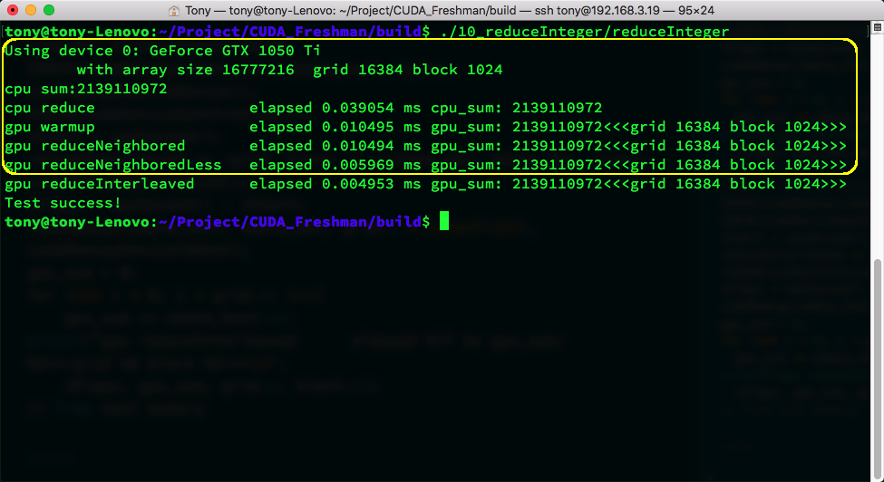
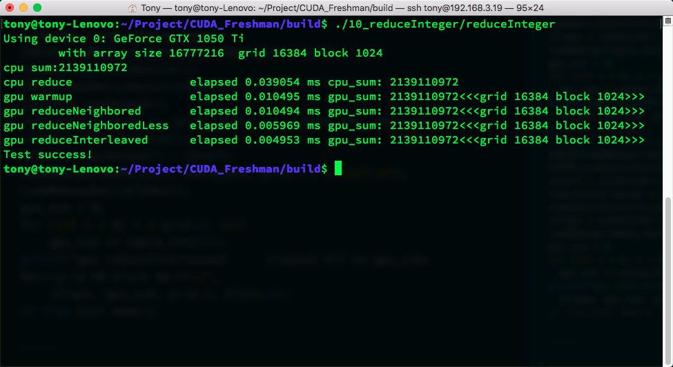
The above image shows execution results. There are so many because I've also included the two optimized versions below. The yellow box shows our code's execution result and time. warmup is used to start the GPU beforehand to prevent first-launch overhead from affecting efficiency tests. warmup's code is the same as reduceNeighbored -- there's still a slight difference.
Improving Parallel Reduction Divergence
The reduction above is obviously the most primitive form. Unoptimized code shouldn't be used in production. Or rather, a truth: nobody can write satisfactory code on the first try.
if ((tid % (2 * stride)) == 0)
This conditional creates massive branching in the kernel, as shown:
- Round 1: 1/2 of threads are unused
- Round 2: 3/4 of threads are unused
- Round 3: 7/8 of threads are unused
Thread utilization is very low. Since these threads are in the same warp, they can only wait -- they can't execute other instructions.
For this low utilization, we came up with the following solution:
Note that the numbers inside the orange circles are thread indices. This computation pattern has higher thread utilization than the original version. The kernel function is:
__global__ void reduceNeighboredLess(int * g_idata, int *g_odata, unsigned int n)
{
    unsigned int tid = threadIdx.x;
    unsigned idx = blockIdx.x * blockDim.x + threadIdx.x;
    // convert global data pointer to the local point of this block
    int *idata = g_idata + blockIdx.x * blockDim.x;
    if (idx > n)
        return;
    //in-place reduction in global memory
    for (int stride = 1; stride < blockDim.x; stride *= 2)
    {
        //convert tid into local array index
        int index = 2 * stride * tid;
        if (index < blockDim.x)
        {
            idata[index] += idata[index + stride];
        }
        __syncthreads();
    }
    //write result for this block to global mem
    if (tid == 0)
        g_odata[blockIdx.x] = idata[0];
}
The most critical step is:
int index = 2 * stride * tid;
This step ensures index can move forward to memory positions with data to process, rather than simply mapping tid to memory addresses, which causes many threads to be idle.
So where's the efficiency advantage?
First, we ensure that in a block, the first few executing warps run at near-full capacity, while the latter half of the warps essentially don't need to execute. When a warp has branches and neither branch needs to execute, the hardware stops scheduling them, saving resources. That's where the efficiency comes from. If all non-matching branches still had to execute even when an entire warp didn't need to, this approach would be ineffective. Fortunately, modern hardware is smart enough. After execution, we get:
The efficiency improvement is astounding -- it dropped a whole decimal place, roughly halving the time.
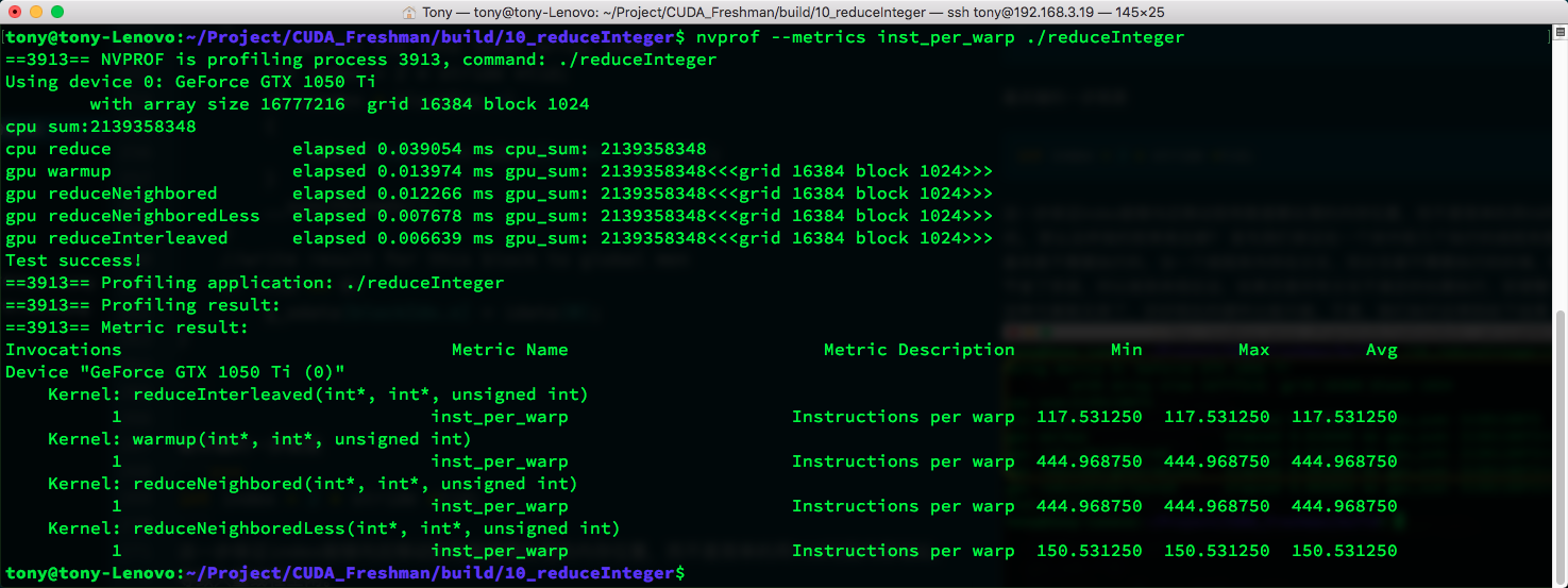
We've been introducing a tool called nvprof. Let's now look at the average number of instructions executed per warp. I'll give results for all four kernels, but we only care about the yellow box.
Using the following command:
nvprof --metrics inst_per_warp ./reduceInteger
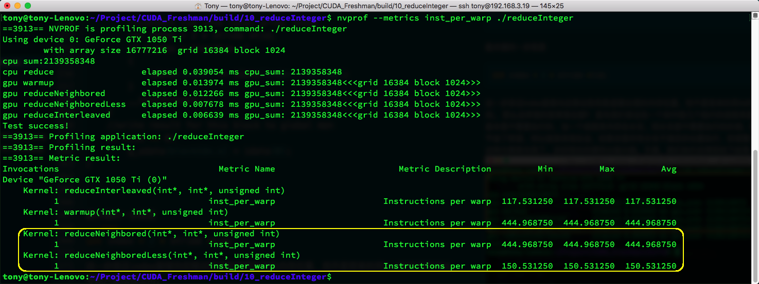
The metric shows the original kernel at 444.9 vs. the new kernel at 150.5. Clearly, the original kernel executed many branch instructions that were meaningless.
The higher the divergence, the higher the inst_per_warp metric. Remember this -- we'll use it frequently when testing efficiency.
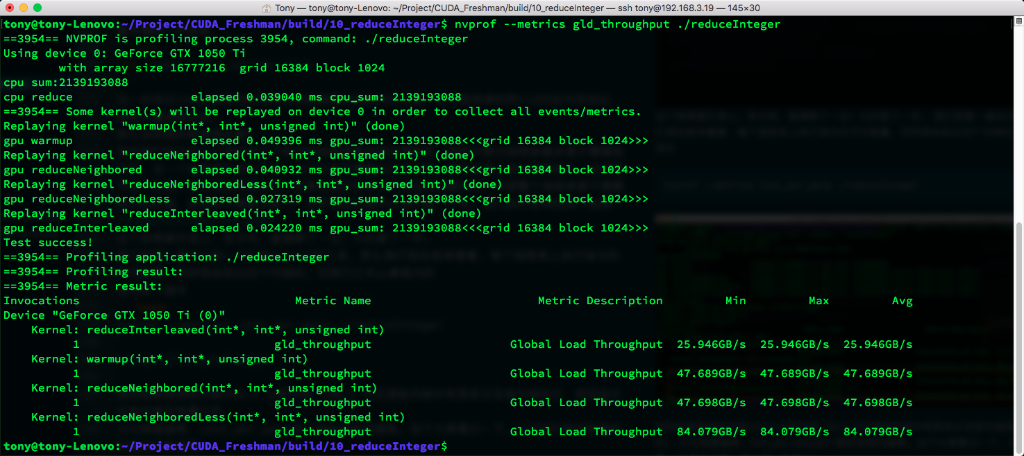
Next, let's look at memory load throughput:
nvprof --metrics gld_throughput ./reduceInteger
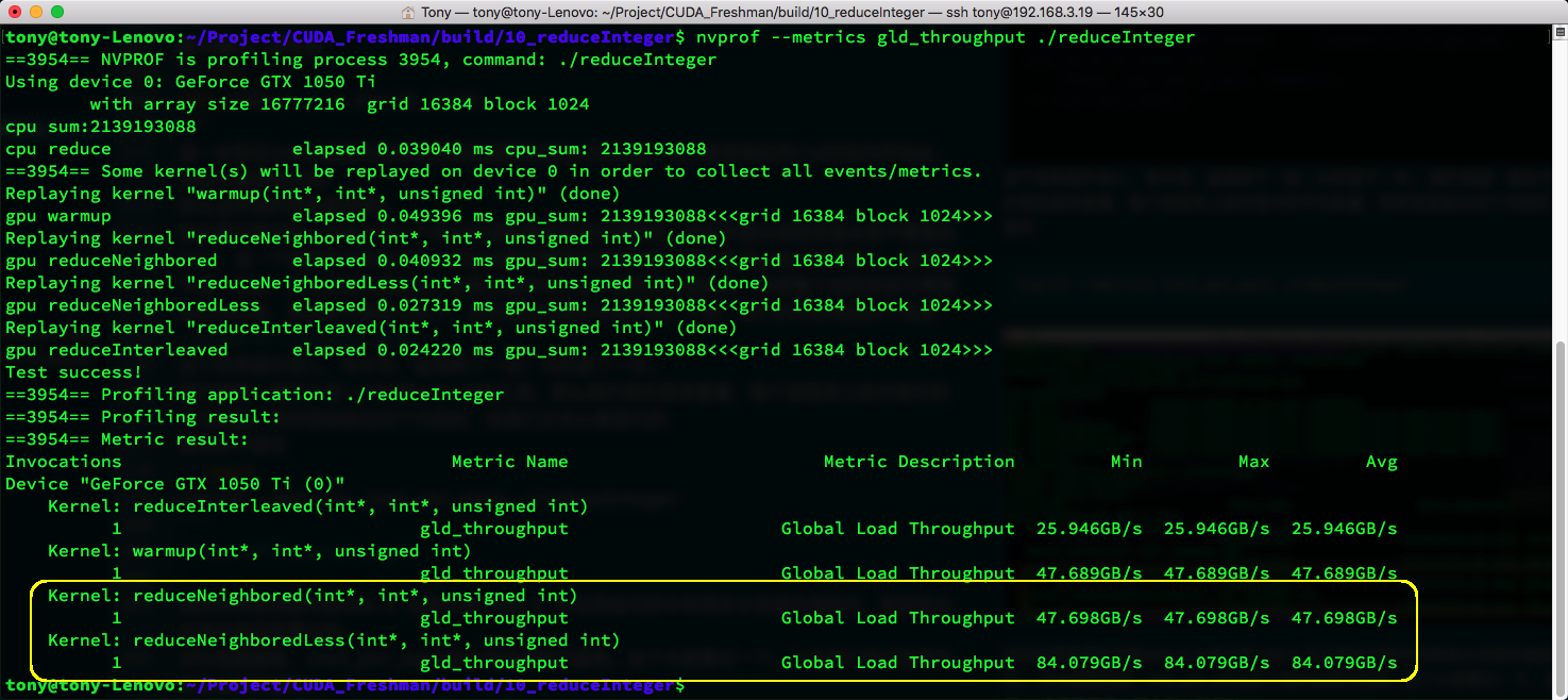
Again, just look at the yellow box. Our new kernel has much higher memory efficiency, also nearly doubled. The reason is what we analyzed above: in a thread block, the first few warps are working while the latter ones don't work at all. The ones not working aren't scheduled, and the ones working have concentrated memory requests, maximizing bandwidth utilization. In the naive kernel, non-working threads still run within their warp without requesting memory, fragmenting memory access. Theoretically, only half the memory efficiency is achieved, and testing confirms this closely.
Interleaved Reduction
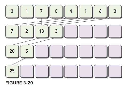
The approach above modifies which data threads process to maximize utilization of certain warps. Next, we use the same idea but a different method: we adjust the stride. Each thread still processes its corresponding memory position, but the memory pairs are no longer adjacent -- they're separated by a certain distance:
A diagram is the best way to describe this:
We still treat the diagram as a complete thread block. The first half of the warps run at maximum load, while the latter half do no work.
__global__ void reduceInterleaved(int * g_idata, int *g_odata, unsigned int n)
{
    unsigned int tid = threadIdx.x;
    unsigned idx = blockIdx.x * blockDim.x + threadIdx.x;
    // convert global data pointer to the local point of this block
    int *idata = g_idata + blockIdx.x * blockDim.x;
    if (idx >= n)
        return;
    //in-place reduction in global memory
    for (int stride = blockDim.x/2; stride > 0; stride >>= 1)
    {
        if (tid < stride)
        {
            idata[tid] += idata[tid + stride];
        }
        __syncthreads();
    }
    //write result for this block to global mem
    if (tid == 0)
        g_odata[blockIdx.x] = idata[0];
}
Execution result:
From an optimization principle perspective, this kernel should have the same efficiency as the previous one. But the test results show this new kernel is significantly faster than the previous one. Let's examine the metrics:
nvprof --metrics inst_per_warp ./reduceInteger
nvprof --metrics gld_throughput ./reduceInteger
reduceInterleaved has the lowest memory efficiency, but the least warp divergence.
The book says reduceInterleaved's advantage is in memory reads, not warp divergence. But our actual experiments yielded completely different conclusions. Is memory to blame, or is the compiler at fault? Stay tuned for our next series, where we'll directly examine machine code to determine what actually affects these two kernels that appear similar but have vastly different results.
Machine code inspection needed to determine the actual differences between the two kernels.
Summary
This article is somewhat embarrassing -- the final conclusion contradicts the book. But the overall thinking flow is still smooth, so I'm publishing it anyway. Normally, I wouldn't publish something with unresolved questions (unable to determine if existing technology can solve it), but considering it might be due to compiler evolution, I'm publishing it first. If I figure it out later, it'll be discussed as a case study in the CUDA Advanced series.