2.2 Timing Kernel Functions

2018-03-08 | CUDA , Freshman | 0 |

Abstract: This article introduces CUDA kernel function timing methods. Keywords: gettimeofday, nvprof

Timing Kernel Functions

In the programming model section, we covered memory and thread-related knowledge, and then we launched our kernel function. These only roughly outline the appearance of CUDA programming. Through the previous articles, you can write general runnable programs, but to achieve the highest efficiency, repeated optimization and detailed understanding of hardware and programming details are needed. How do we evaluate efficiency? Time is a very intuitive measurement.

Timing with the CPU

Using the CPU to time is a common method for testing execution time. The most commonly used timing method when writing C programs is:

clock_t start, finish;
start = clock();
// part to test
finish = clock();
duration = (double)(finish - start) / CLOCKS_PER_SEC;

Here, clock() is a key function. The time measured by the clock function is the process running time, in units of ticks. Literally, the CLOCKS_PER_SEC macro means how many clocks per second -- the value may differ across systems. It's important to note that this timing method has serious issues with parallel programs! If you want to know the exact reason, you can look up the clock source code (a standard C language function).

Here we use the gettimeofday() function:

#include <sys/time.h>
double cpuSecond()
{
    struct timeval tp;
    gettimeofday(&tp, NULL);
    return ((double)tp.tv_sec + (double)tp.tv_usec * 1e-6);
}

gettimeofday is a library function on Linux that returns the number of seconds since midnight January 1, 1970. It requires the header file sys/time.h.

Now let's use this function to test kernel function execution time:

I'll paste the code section here. For the complete code, visit the repository: https://github.com/Tony-Tan/CUDA_Freshman

#include <cuda_runtime.h>
#include <stdio.h>
#include "freshman.h"

__global__ void sumArraysGPU(float *a, float *b, float *res, int N)
{
    int i = blockIdx.x * blockDim.x + threadIdx.x;
    if(i < N)
        res[i] = a[i] + b[i];
}

int main(int argc, char **argv)
{
    // set up device.....
    
    // init data ......
    
    // timer
    double iStart, iElaps;
    iStart = cpuSecond();
    sumArraysGPU<<<grid, block>>>(a_d, b_d, res_d, nElem);
    cudaDeviceSynchronize();
    iElaps = cpuSecond() - iStart;
    
    // ......
}

Let's mainly analyze the timing section. First, iStart is cpuSecond returning a number of seconds. Then the kernel function executes. After the kernel starts executing, control immediately returns to the host thread, so we must add a synchronization function to wait for the kernel to finish. Without this synchronization function, the measured time would be from calling the kernel to the kernel returning to the host thread, not the actual kernel execution time. After adding:

cudaDeviceSynchronize();

The timing measures from calling the kernel function to the kernel finishing execution and returning to the host. The diagram below roughly describes the different time points in the execution process:

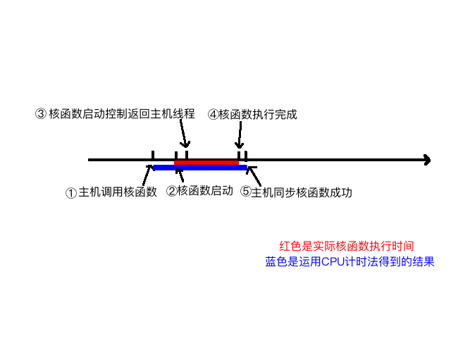
We can roughly analyze the process from kernel launch to completion:

1. Host thread launches the kernel
2. Kernel launches successfully
3. Control returns to the host thread
4. Kernel execution completes
5. Host synchronization function detects kernel execution is complete

What we want to measure is the time from step 2 to 4, but with CPU timing methods, we can only measure the time from step 1 to 5. So the measured time is somewhat longer.

Next, let's adjust our parameters to see the impact of different thread dimensions on speed, and whether timing can reflect the issues. Here we consider a one-dimensional thread model:

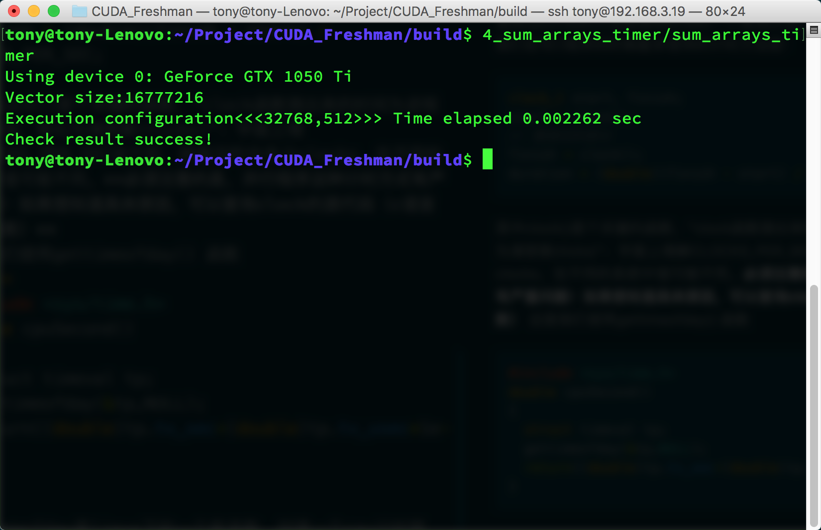
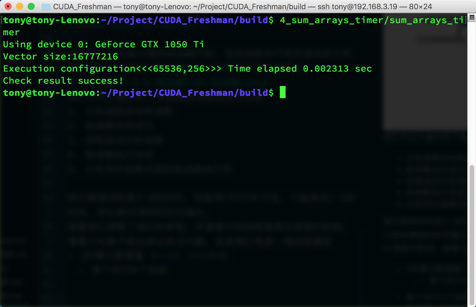
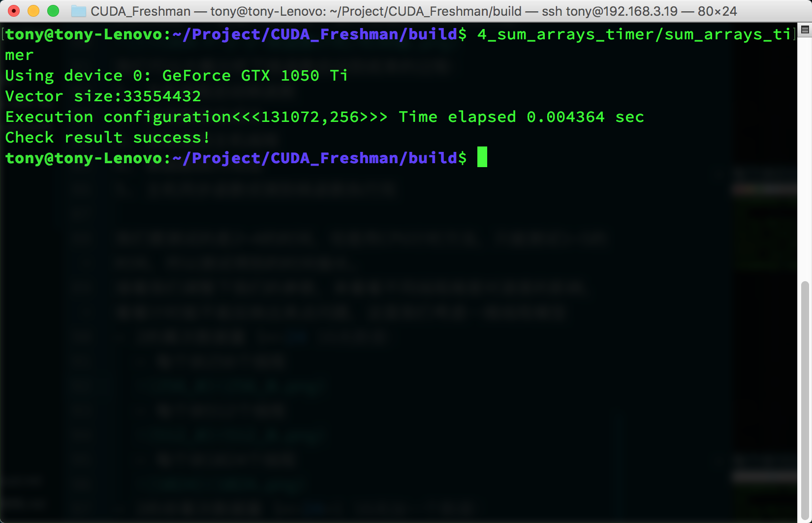
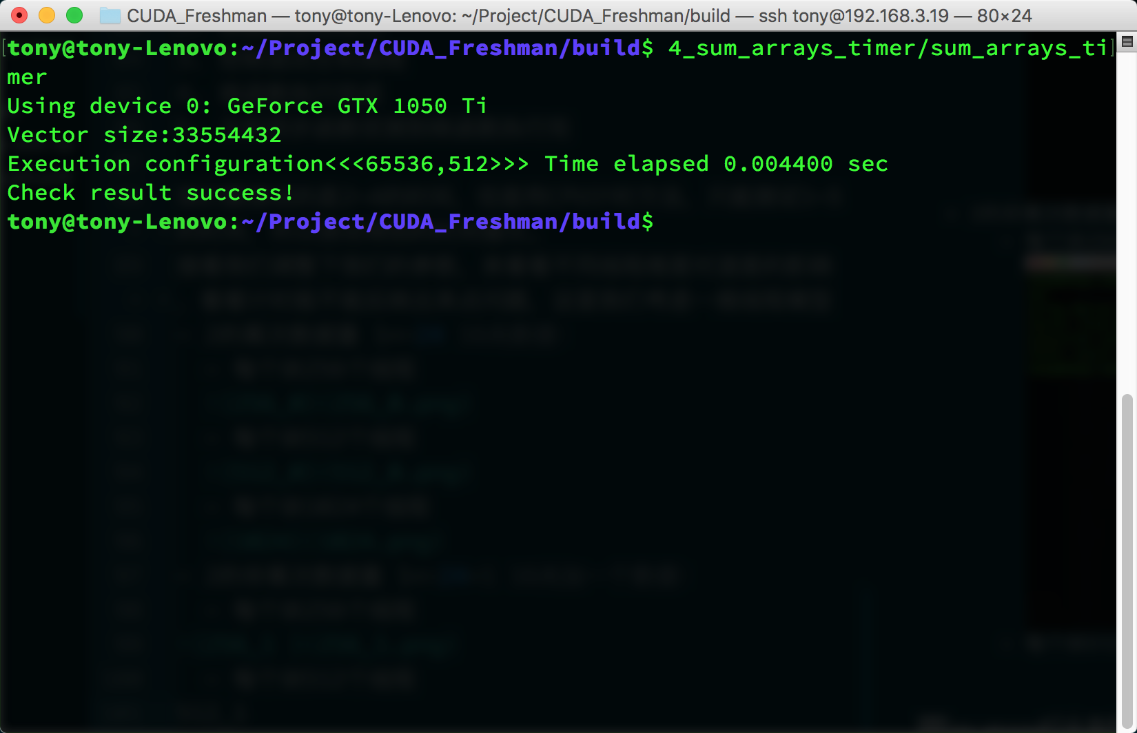
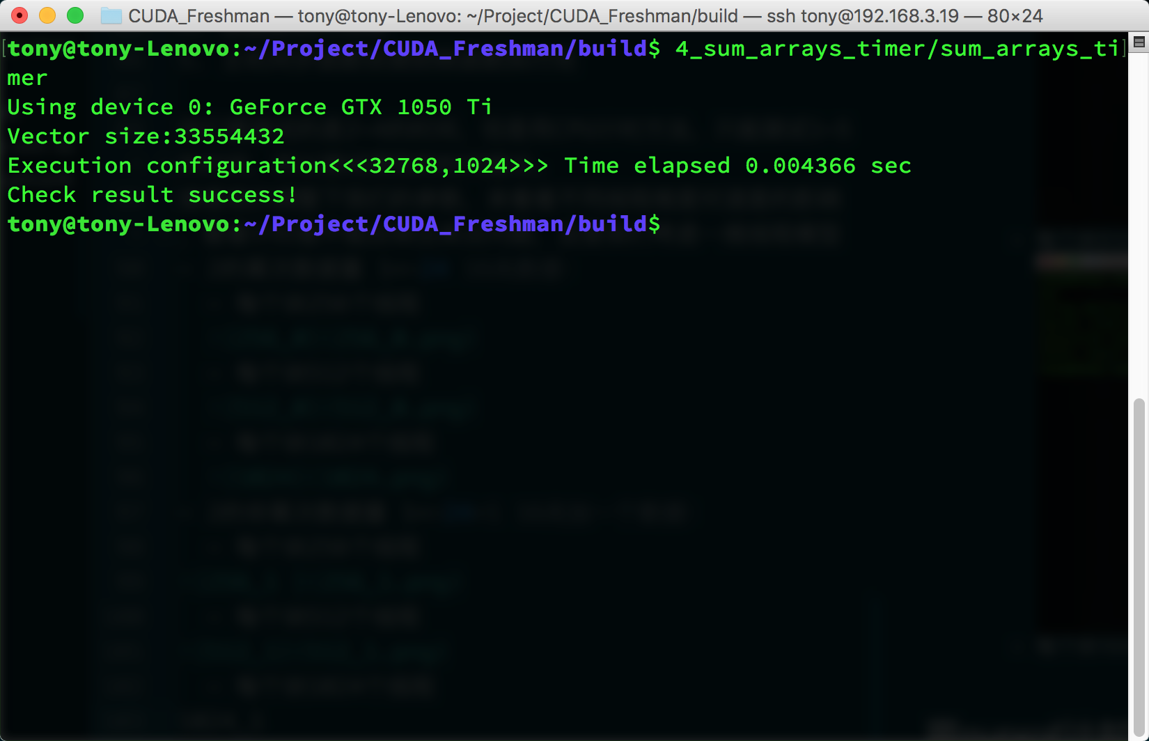
• Power-of-two data size 1<<24, 16M data:

  • 256 threads per block
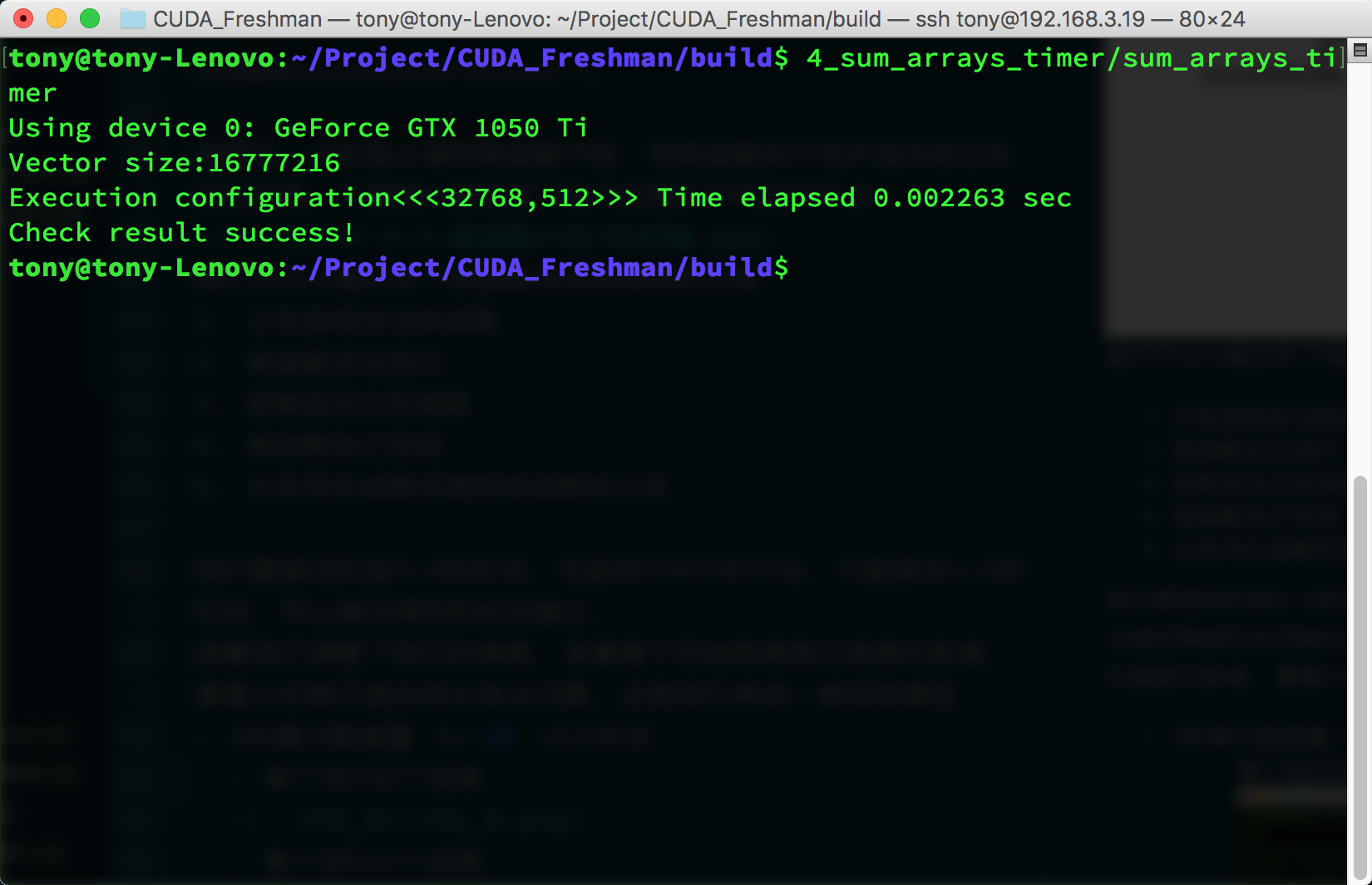
  • 512 threads per block
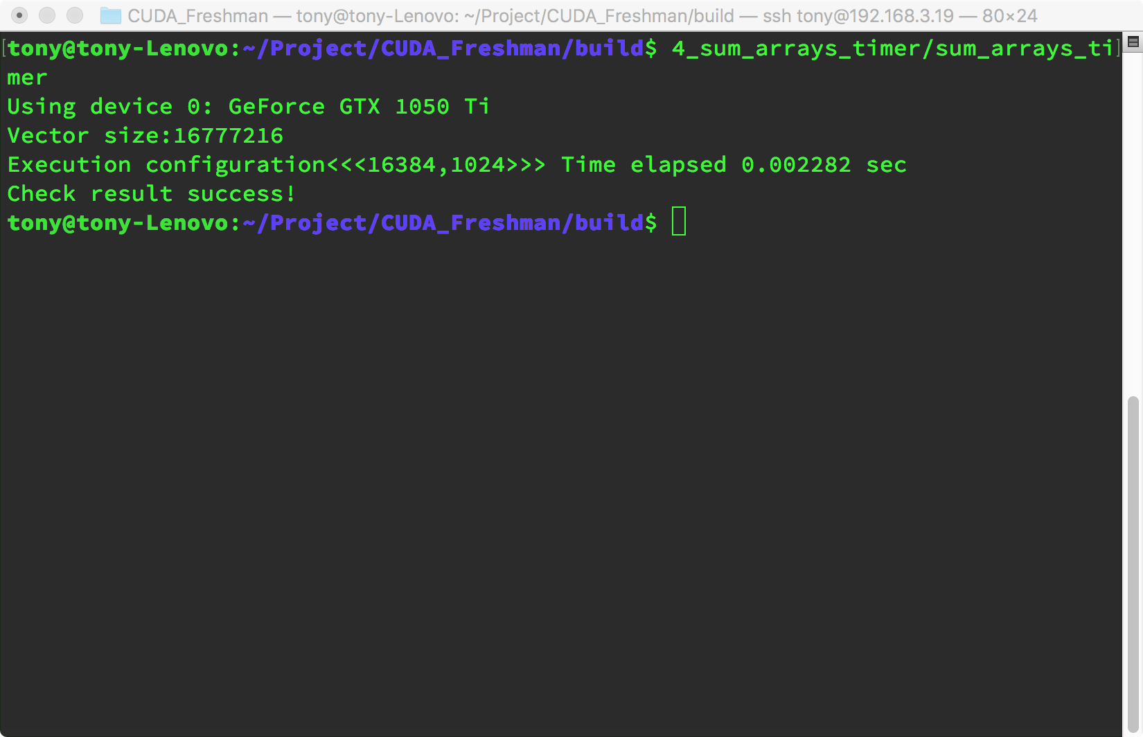
  • 1024 threads per block

• Non-power-of-two data size (1<<24)+1, 16M plus one:

  • 256 threads per block
  • 512 threads per block
  • 1024 threads per block

For this test environment, the performance difference between these three parameters is relatively small. However, it's worth noting that when data can't be evenly divided into complete blocks, performance drops significantly. We can use a small trick here -- for example, only transfer data that can be evenly divided into blocks, then use the CPU for the remaining 1 or 2 elements. This technique will be introduced later, along with how to choose coefficients. In this article, we're only concerned with how the timing function works, and so far it looks good.

Timing with nvprof

After CUDA 5.0, there's a command-line profiling tool called nvprof. We'll also introduce a graphical tool later. For now, let's learn about nvprof. The main trick for learning a tool is to learn all its features -- once you've mastered all the features of a tool, that's when learning is successful.

nvprof usage:

$ nvprof [nvprof_args] <application> [application_args]

On some systems, you may encounter a permissions error:

======== Error: unified memory profiling failed.

The reason is a permissions issue. For security reasons, on macOS and Linux, when debugging a program that needs to attach to another process, permissions are required to ensure security; otherwise, malicious programs could interfere with other programs. The solution is to use sudo:

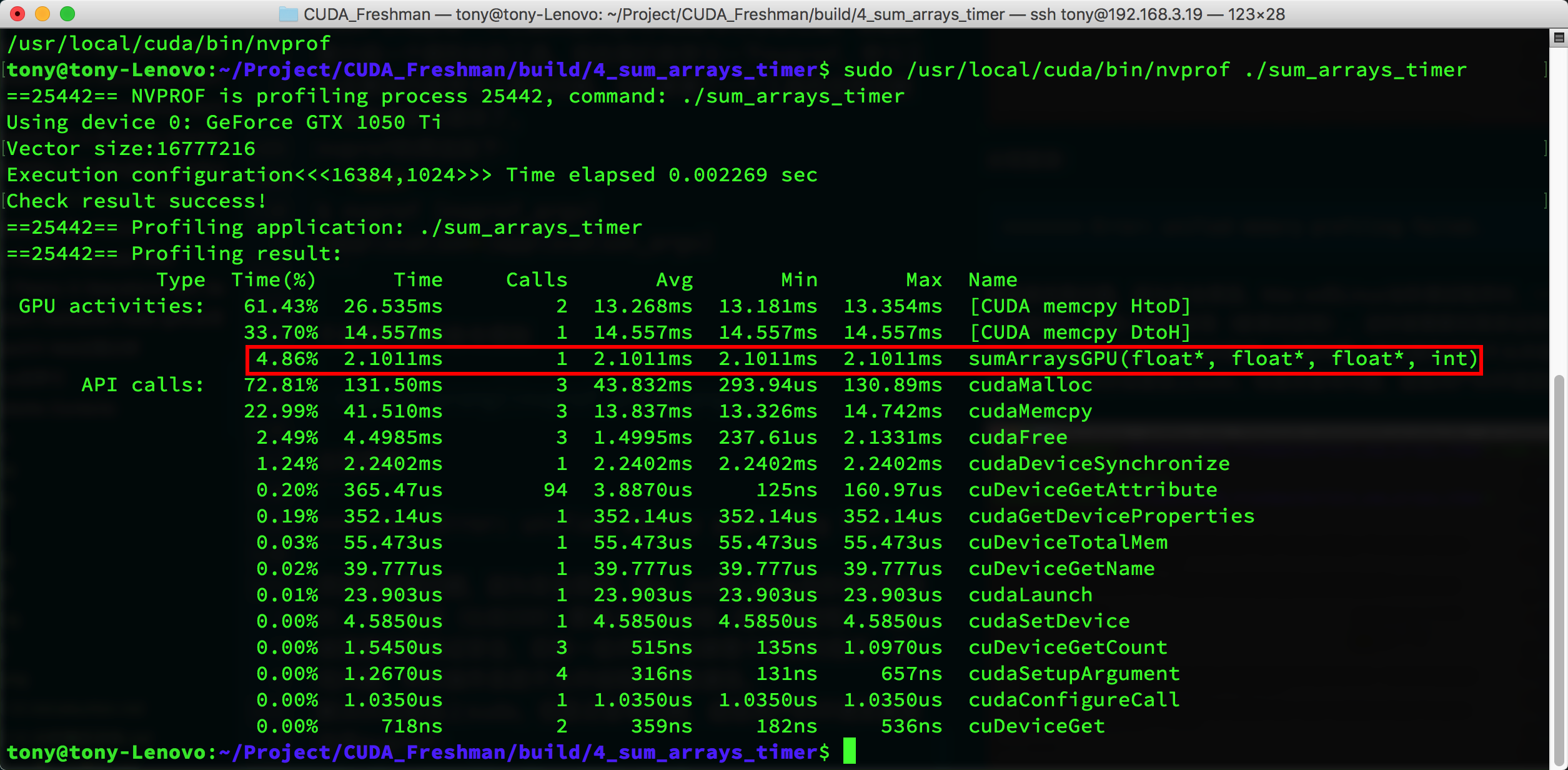
The tool not only gives kernel execution time and proportion but also the execution time of other CUDA functions. You can see that kernel execution time is only about 4%, while other operations like memory allocation and memory copy take up most of the time. The kernel execution time given by nvprof is 2.1011ms, while the cpuSecond timing result above is 2.282ms. This shows that nvprof is likely closer to the actual value.

nvprof is a powerful tool that gives us optimization targets. Analyzing the data helps us determine where to focus our efforts.

Theoretical Performance Limit

Having obtained actual operation values, we need to know the limit of what we can optimize -- that is, the machine's theoretical computation limit. We can never reach this limit, but we must know it clearly. For example, if the theoretical limit is 2 seconds and we've already optimized from 10 seconds to 2.01 seconds, there's essentially no need to spend a lot of time further optimizing speed. Instead, we should consider buying more machines or newer equipment.

The theoretical limits of each device can be calculated from its chip specifications. For example:

Tesla K10 Calculation Example:

• Single-precision peak floating-point operations:

  745MHz core frequency x 2 GPUs/chip x (8 multiprocessors x 192 FP units x 32 cores/multiprocessor) x 2 OPS/cycle = 4.58 TFLOPS

• Peak memory bandwidth:

  2 GPUs/chip x 256 bits x 2500MHz memory clock x 2 DDR / 8 bits/byte = 320 GB/s

• Compute intensity:

  4.58 TFLOPS / 320 GB/s = 13.6 instructions : 1 byte

Summary

In this article, we briefly introduced CUDA kernel function timing methods and how to evaluate the theoretical lower bound of execution time -- the efficiency limit. Understanding performance bottlenecks and performance limits is the first step in optimizing performance.