3.2 Understanding the Essence of Warp Execution (Part II)

2018-03-15 | CUDA , Freshman | 0 |

Abstract: This article introduces the second half of the CUDA warp execution essence, covering resources, latency, synchronization, scalability, and other factors that seriously affect performance: throughput, bandwidth, occupancy, and CUDA synchronization. Keywords: Warp Execution, Resource Allocation, Latency Hiding, Occupancy, CUDA Synchronization

Understanding the Essence of Warp Execution (Part II)

These recent articles should be the most core part of CUDA -- not the programming model, but the execution model. Through the execution model, we understand the specific operating mode of GPU hardware, which ensures we can write faster and better programs.

Resource Allocation

As we mentioned earlier, the basic unit of execution on each SM is the warp. That is, a single instruction is broadcast to all threads of a warp through the instruction dispatcher. These threads execute the same command at the same time -- of course, there are branch situations, which we covered in the previous article. That's the executing part. But there are many warps not executing -- what about them? I've divided them into two categories (note: this is my own classification; it may not match official terminology). Moving away from the perspective within a warp (where we observe thread behavior; leaving the warp level lets us observe warp behavior): one type is already activated, meaning these warps are actually ready on the SM, just waiting for their turn -- their state is called blocked. The other type may be assigned to the SM but hasn't made it onto the chip yet -- I call these inactive warps.

How many warps are in the activated state on each SM depends on the following resources:

• Program counters
• Registers
• Shared memory

Once a warp is activated and arrives on-chip, it will not leave the SM until execution completes.

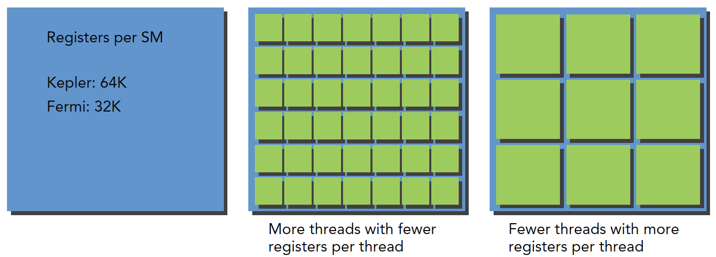
Each SM has 32-bit register sets. The number of registers differs across architectures. They're stored in the register file and allocated for each thread. Meanwhile, a fixed amount of shared memory is allocated among thread blocks.

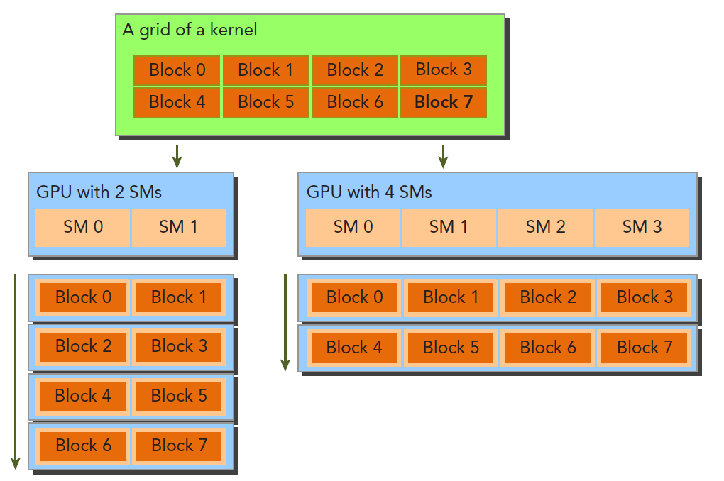
How many thread blocks and warps are assigned to an SM depends on the available registers and shared memory in the SM, as well as the registers and shared memory the kernel requires.

This is a balancing problem. Like a fixed-size container, how many items it can hold depends on the container's size and the items' size. Compared to a large container, a small container might hold ten small items or two large items. SM resources work the same way: when a kernel uses fewer resources, more threads (and thus more warps) can be in the active state, and vice versa.

Regarding register resource allocation:

Regarding shared memory allocation:

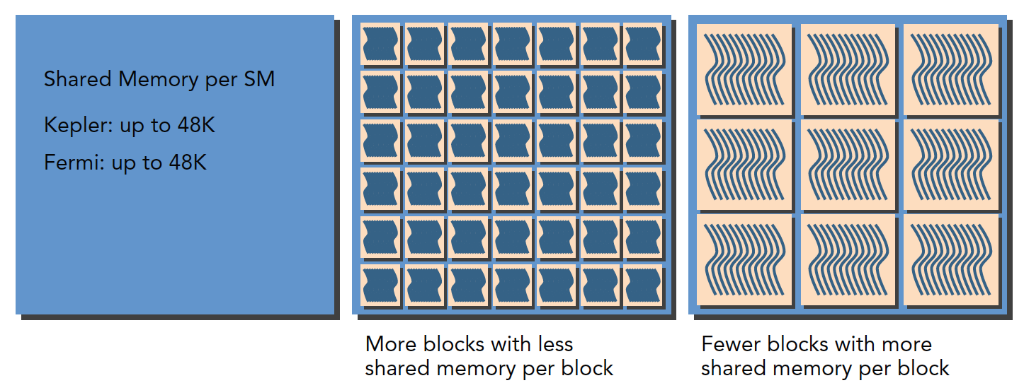
The above mainly discusses warps. If we look at thread blocks logically, the allocation of available resources also affects the number of resident thread blocks.

In particular, if the resources within an SM can't accommodate a complete block, the program won't be able to start. This is something we should check ourselves -- how large is the kernel, or how many threads per block, for this situation to occur.

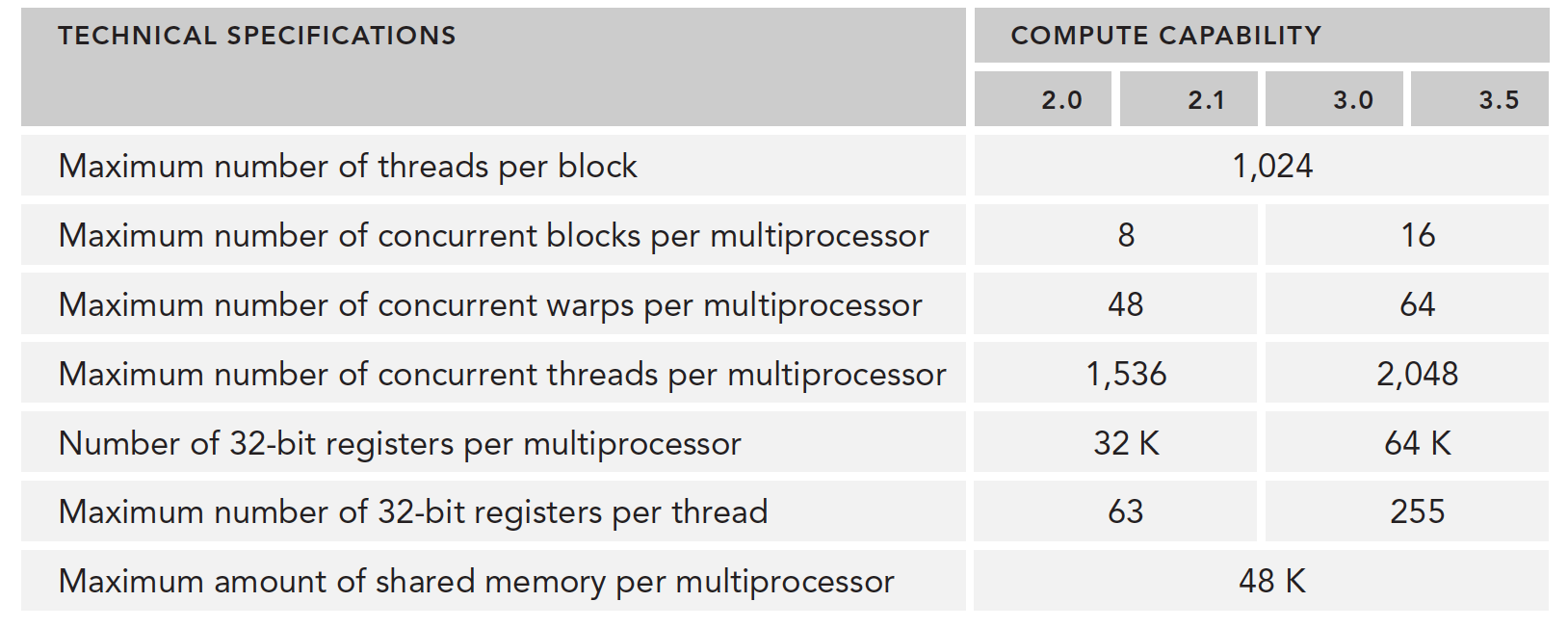
Here is a resource list:

When registers and shared memory are allocated to a thread block, that block is in the active state. The warps it contains are called active warps.

Active warps are further divided into three categories:

• Selected warps
• Blocked warps
• Eligible warps

When an SM is about to execute a warp, the warp being executed is called the selected warp. Those ready to execute are called eligible warps. If a warp doesn't meet the conditions and isn't ready, it's a blocked warp.

A warp must meet the following requirements to be considered eligible:

• 32 CUDA cores are available for execution
• All required resources are in place

The number of active warps on Kepler must not exceed 64 from start to finish (can equal 64). At any cycle, the number of selected warps is less than or equal to 4. Since computing resources are shared among warps, and warps remain on-chip throughout their entire lifecycle, warp context switching is extremely fast.

Below we'll introduce how to hide latency through a large number of active warp switches.

Latency Hiding

Latency hiding -- what is latency? It's the time computation takes when you ask a computer to calculate something. A macroscopic example: say you give a computer an algorithm verification task. It assigns a specific computing unit to complete it, taking ten minutes. During those ten minutes, you wait -- you can only compute the next task after it finishes. The computer's utilization during those ten minutes might not be 100% -- meaning some of its functions are idle. You wonder: can I run another program with different data? (Those with machine learning experience won't find this unfamiliar -- everyone runs multiple versions simultaneously.) You have the computer run it, and find resources still aren't fully utilized, so you keep adding tasks. By the ten-minute mark, you've added ten tasks and still haven't finished adding, but the first task has completed. If you stop adding tasks now and wait for all subsequent tasks to finish, the total time is 20 minutes for 10 tasks -- average time per task: 20/10 = 2 minutes/task. But we have another scenario: since there are many more tasks, at the ten-minute mark when the first task finishes, you continue adding tasks. This cycle continues. At twenty minutes, you stop adding tasks and wait until thirty minutes for all tasks to complete. Average time per task: 30/20 = 1.5 minutes/task. If you keep adding: lim(n->infinity) (n+10)/n = 1 -- the limit speed is one minute per task, hiding 9 minutes of latency.

Of course, another important parameter above is the rate of adding tasks: 10 per ten minutes. If you could add 100 per ten minutes, then in twenty minutes you'd execute 100 tasks, each taking: 20/100 = 0.2 minutes/task. Thirty minutes: 30/200 = 0.15. If you keep adding: lim(n->infinity) (n+10)/(n x 10) = 0.1 minutes/task.

This is the ideal scenario. One thing that must be considered: although you added 100 tasks in ten minutes, the computer might be fully loaded after 50. In that case, the limit speed is only: lim(n->infinity) (n+10)/(n x 5) = 0.2 minutes/task.

So the goal of maximization is to maximize hardware utilization, especially the compute hardware running at full capacity. If nobody is idle, utilization is highest. When some are idle, utilization drops significantly. In other words, maximize the utilization of functional units. Utilization is directly related to the number of resident warps.

The hardware thread scheduler is responsible for scheduling warps. When there are always available warps for it to schedule, compute resources can be fully utilized. Through instructions issued from other resident warps, the latency of each instruction can be hidden.

Compared to other types of programming, latency hiding is extremely important for GPUs. Instruction latency is generally divided into two types:

• Arithmetic instruction latency
• Memory instruction latency

Arithmetic instruction latency is the time between when an arithmetic operation starts and when it produces a result. During this time, only certain computing units are working, while other logic units are idle.

Memory instruction latency is easy to understand: when a memory access occurs, computing units must wait for data to be fetched from memory to registers. This cycle is very long.

Latency:

• Arithmetic latency: 10-20 clock cycles
• Memory latency: 400-800 clock cycles

The diagram below shows the logic flow from blocked warp to eligible warp:

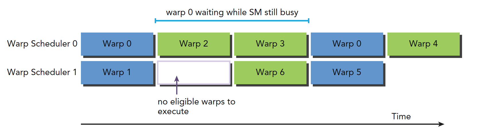
Warp 0 recovers to eligible mode after being blocked for a time, but during this waiting period, the SM is not idle.

How many threads and warps are needed to minimize latency?

Little's Law gives us the following formula:

Warps Required = Latency x Throughput

Note the difference between bandwidth and throughput. Bandwidth generally refers to the theoretical peak -- the maximum number of instructions executable per clock cycle. Throughput refers to the actual number of instructions processed per minute during operation.

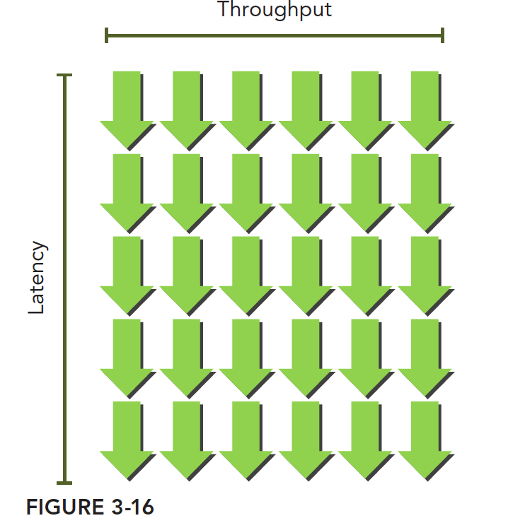
This can be imagined as a waterfall. Like this -- the green arrows are warps. As long as there are enough warps, throughput won't decrease:

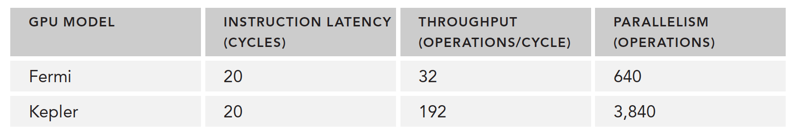
The table below gives the number of parallel operations needed for Fermi and Kepler to execute a simple computation:

There are also two methods to increase parallelism:

• Instruction-Level Parallelism (ILP): A thread has many independent instructions
• Thread-Level Parallelism (TLP): Many concurrent eligible threads

Similarly, just as instruction cycle latency hiding uses the full compute resources, memory read latency hiding aims to use the full memory bandwidth. During memory latency, compute resources are being used by other warps. So we don't consider what compute resources are doing during memory read latency -- these two types of latency are like two different departments following the same principles.

Our fundamental goal is to fully utilize both compute resources and memory bandwidth resources. This achieves theoretical maximum efficiency.

The table below, based on Little's Law, shows how many warps are needed to minimize memory read latency. There's a unit conversion process here: the machine's performance metric for memory speed is given in GB/s, but we need bytes per clock cycle. So we divide this speed by frequency. For example, the M2070's memory bandwidth is 144 GB/s, converted to clock cycles: 144 GB/s / 1.566 GHz = 92 B/t, giving us the memory bandwidth per clock cycle.

This gives us the data in the following table:

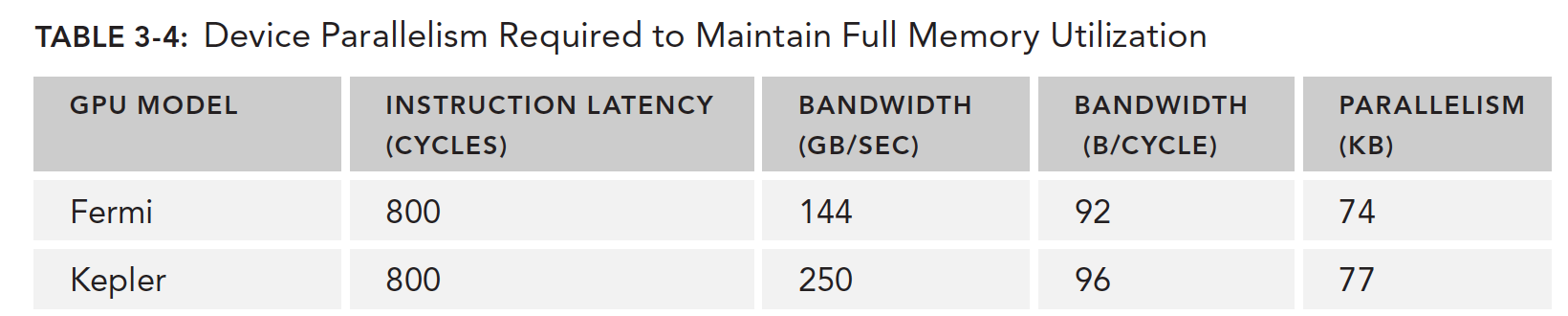
It should be noted that this speed is for the entire GPU device, not a single SM, because we're using the GPU device's memory bandwidth, not an individual SM's.

Fermi needs to read 74KB of data in parallel to fully saturate GPU bandwidth. If each thread reads 4 bytes, we need approximately 18,500 threads -- about 579 warps -- to reach this peak.

So, latency hiding depends on the number of active warps -- the more warps, the better the hiding. But the number of warps is affected by the resources mentioned above. This means we need to find the optimal execution configuration for optimal latency hiding.

How do we determine a lower bound for warps so that when above this number, SM latency is fully hidden? The formula is simple and easy to understand: the SM's compute core count multiplied by the single instruction latency. For example, 32 single-precision floating-point compute units, each with a 20-cycle latency per calculation, means we need at least 32 x 20 = 640 threads to keep the device busy.

Occupancy

Occupancy is the ratio of active warps on an SM to the maximum number of warps supported by that SM. In our earlier program 7_deviceInformation, we can add a few member queries to help find this value:

Complete code: https://github.com/Tony-Tan/CUDA_Freshman

// upper half omitted
printf("----------------------------------------------------------\n");
printf("Number of multiprocessors:                      %d\n", deviceProp.multiProcessorCount);
printf("Total amount of constant memory:                %4.2f KB\n",
       deviceProp.totalConstMem/1024.0);
printf("Total amount of shared memory per block:        %4.2f KB\n",
       deviceProp.sharedMemPerBlock/1024.0);
printf("Total number of registers available per block:  %d\n",
       deviceProp.regsPerBlock);
printf("Warp size                                       %d\n", deviceProp.warpSize);
printf("Maximum number of threads per block:            %d\n", deviceProp.maxThreadsPerBlock);
printf("Maximum number of threads per multiprocessor:  %d\n",
       deviceProp.maxThreadsPerMultiProcessor);
printf("Maximum number of warps per multiprocessor:     %d\n",
       deviceProp.maxThreadsPerMultiProcessor/32);
return EXIT_SUCCESS;

Result:

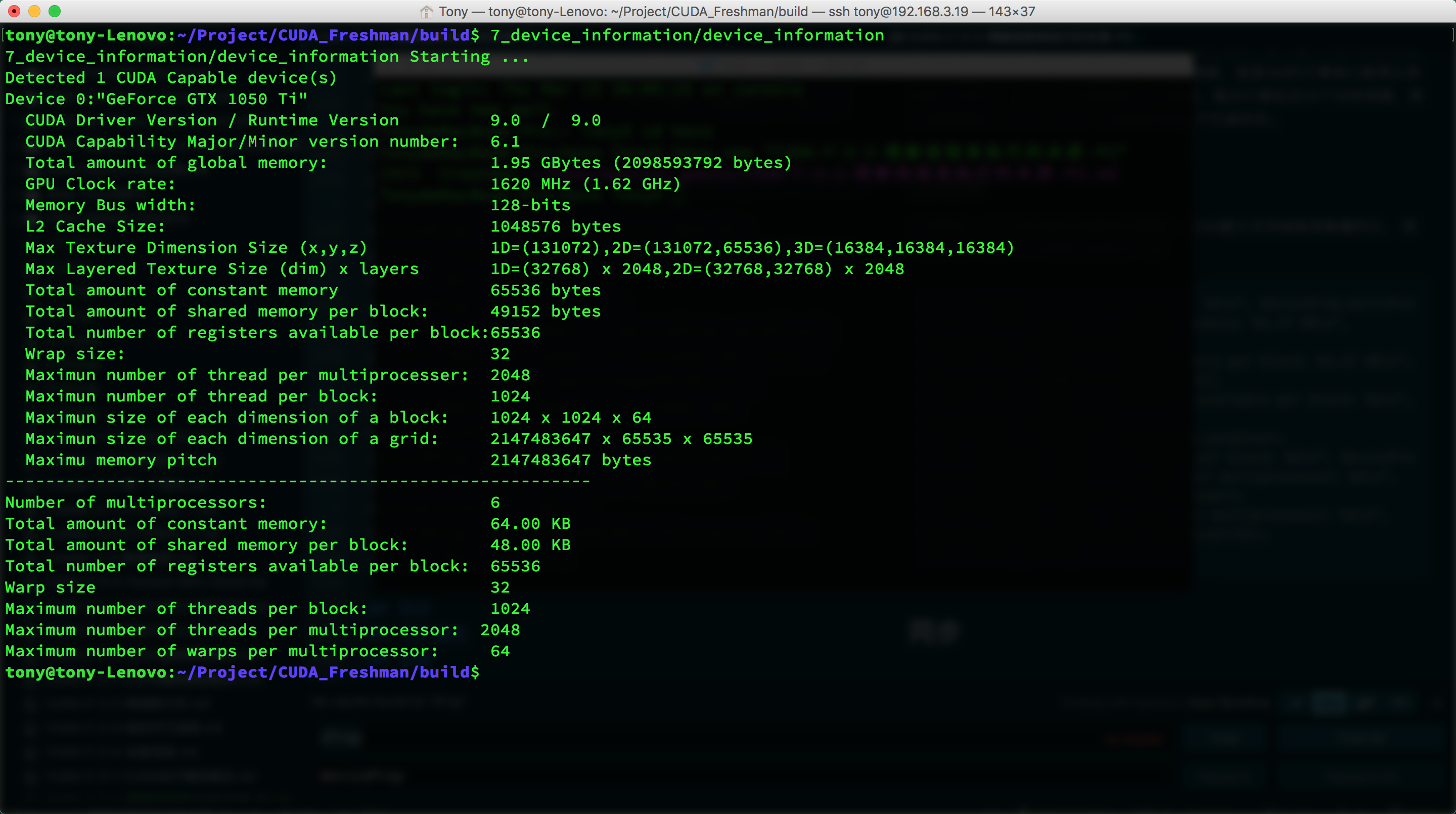
Maximum 64 warps per SM.

The CUDA toolkit provides a spreadsheet called the CUDA Occupancy Calculator. Fill in the relevant data and it will automatically calculate grid parameters for you:

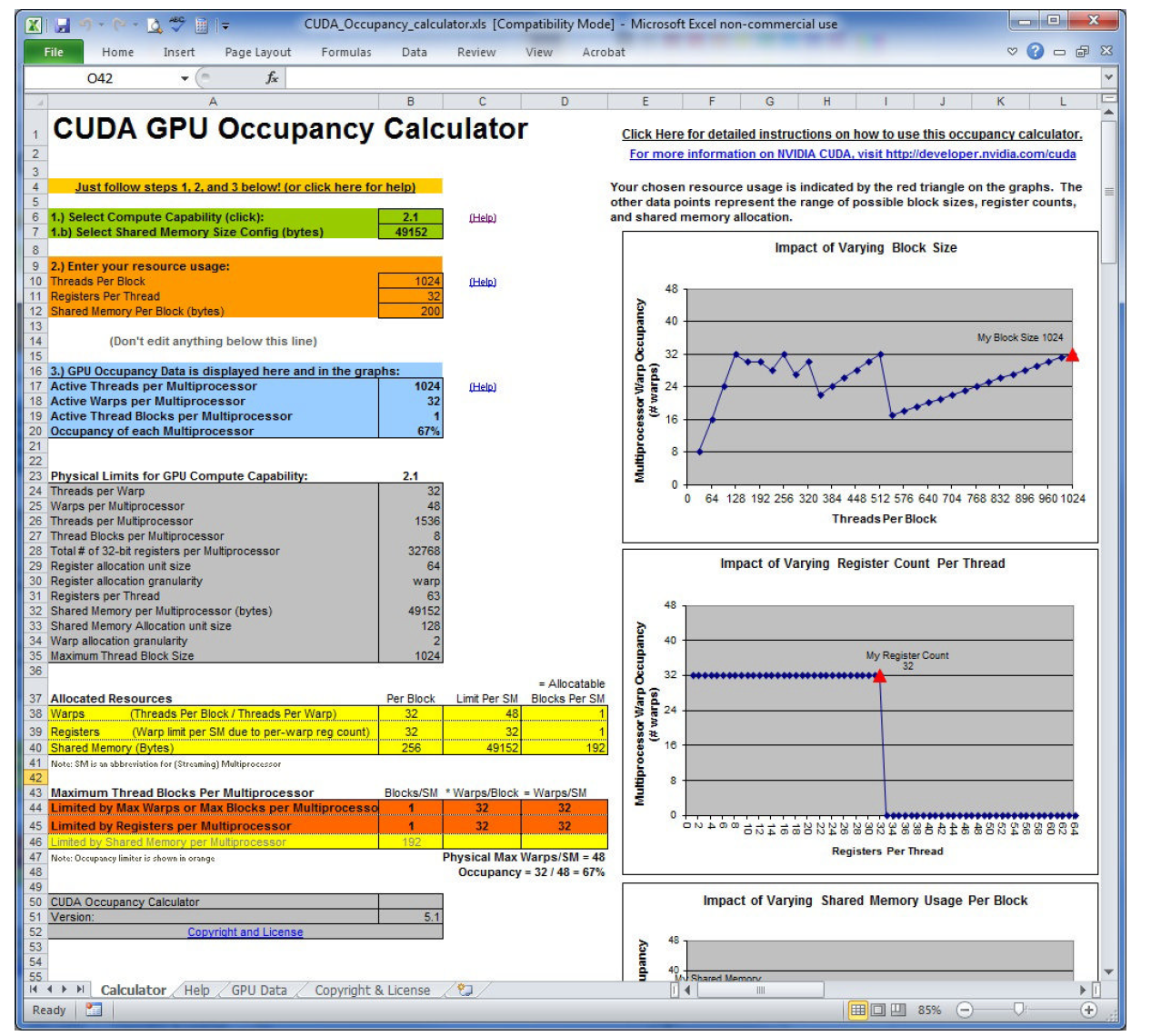
The image above is from the book. A side note: these people actually made a spreadsheet -- why not write a program?

As we've established above, the number of registers a kernel uses affects the number of warps in an SM. nvcc compilation options also allow manual control of register usage.

You can also increase occupancy by adjusting the number of threads per thread block, though it should be reasonable and not extreme:

• Small thread blocks: Too few threads per block will reach the warp maximum before all resources are used up.
• Large thread blocks: Too many threads per block results in fewer hardware resources available per thread in each SM.

Synchronization

Concurrent programs rely heavily on synchronization, such as locks in pthread and synchronization mechanisms in OpenMP. The main purpose is to avoid memory races.

CUDA synchronization covers only two types:

• Intra-thread-block synchronization
• System-level synchronization

Block-level synchronization means all threads within the same block stop at a designated position, using:

__syncthreads();

This function can only synchronize threads within the same block, not across different blocks. To synchronize threads across different blocks, you can only let the kernel function finish executing and return control to the host -- this synchronizes all threads.

Memory races are very dangerous -- be extremely careful. This is a common source of errors.

Scalability

Scalability is relative to different hardware. When a program takes time T on device 1, and device 2 has twice the resources of device 1, we hope to achieve T/2 running time. This property is a feature provided by the CUDA driver. Currently, NVIDIA is dedicated to optimizing this:

Summary

Today was very productive, mainly because this section had already been thoroughly researched. Chapter 3 is the most core part of the Freshman stage. Everyone needs to do more research, more thinking, and more practice. To be continued...