Advanced Mathematics II

[TOC]

Pre-Exam Reminders

When solving integral problems, first check for symmetry.

Then substitute data to see if the integrand equals 1.

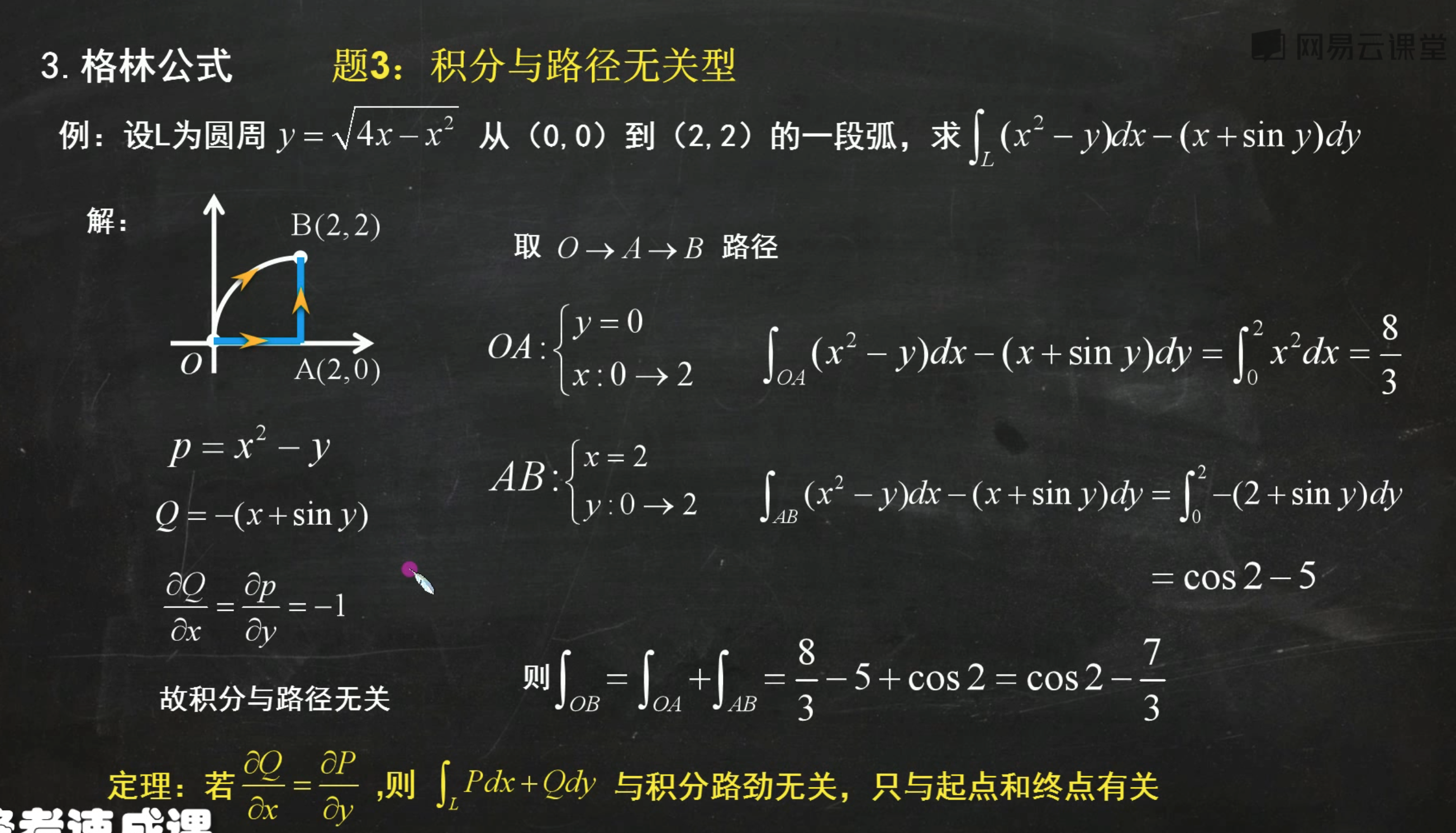
For line integrals of the second kind,

Check if you can use the property that the integral is path-independent.

If the problem mentions exact differential, it means the mixed partial derivatives are equal, and the integral is path-independent.

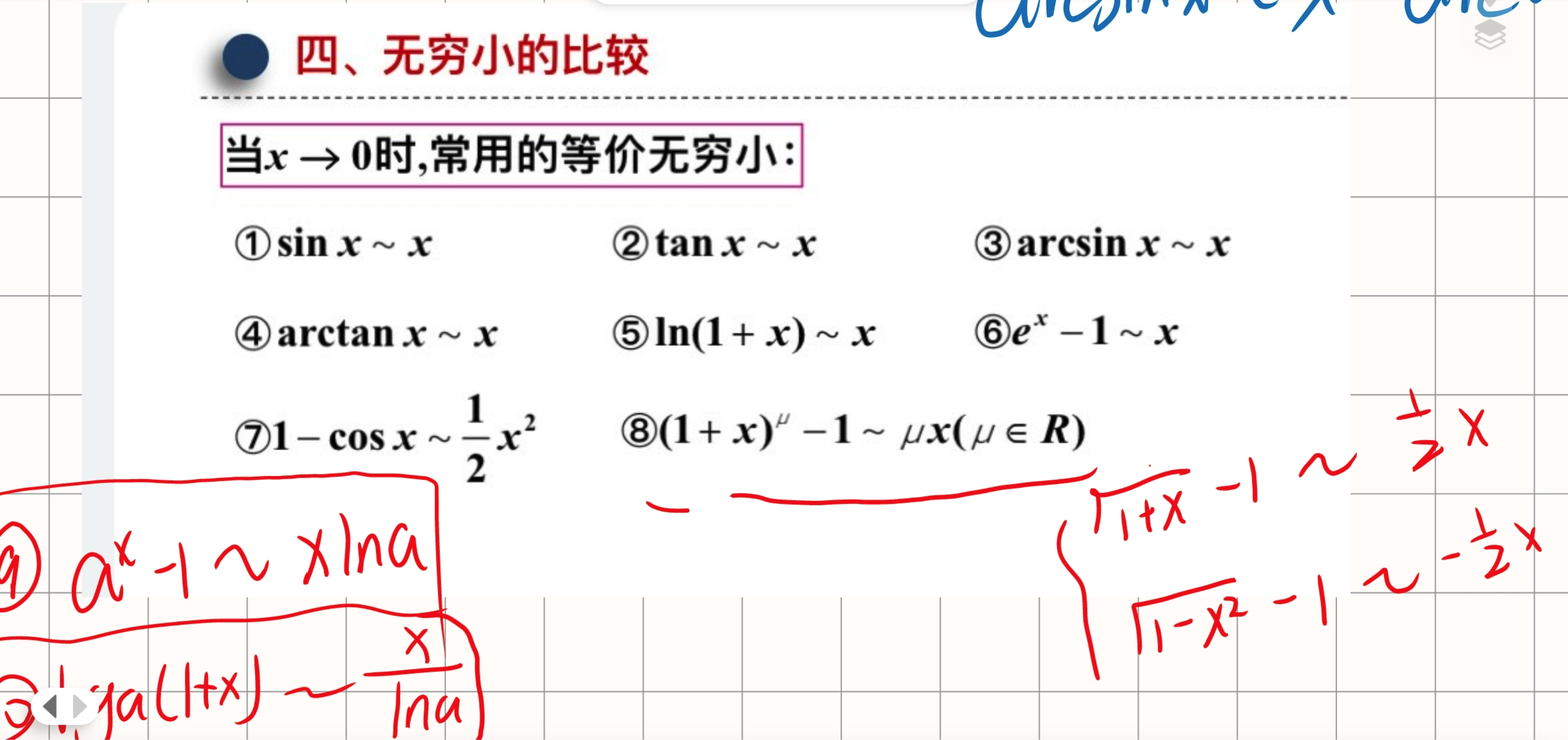
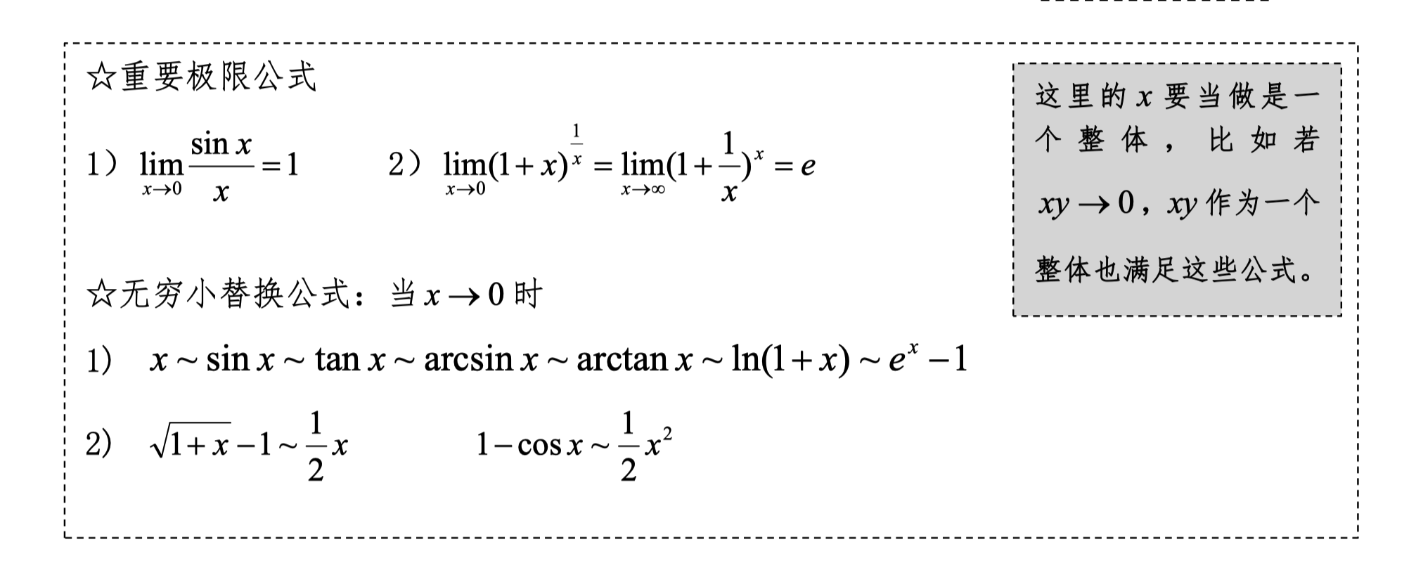
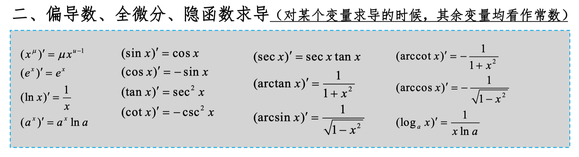
Equivalent Infinitesimals, Derivative Formulas

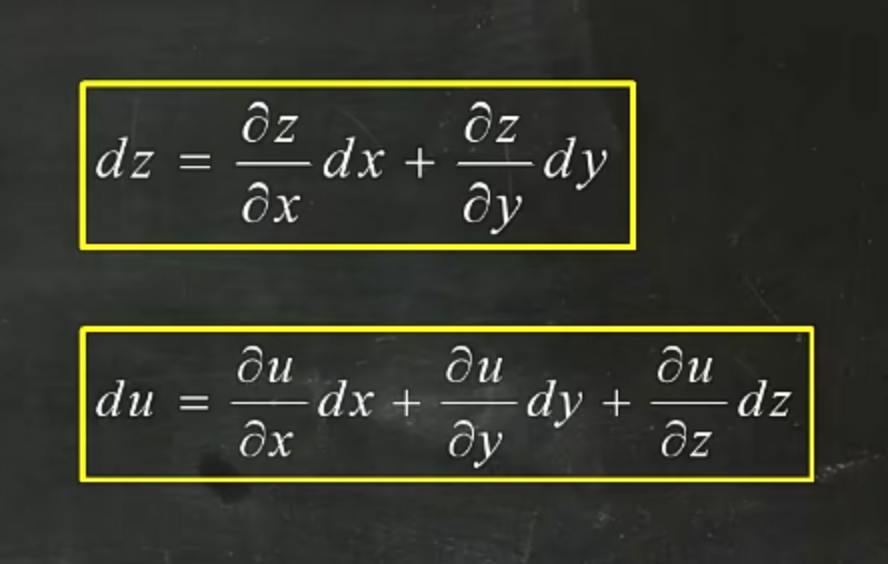
Total Differential Form

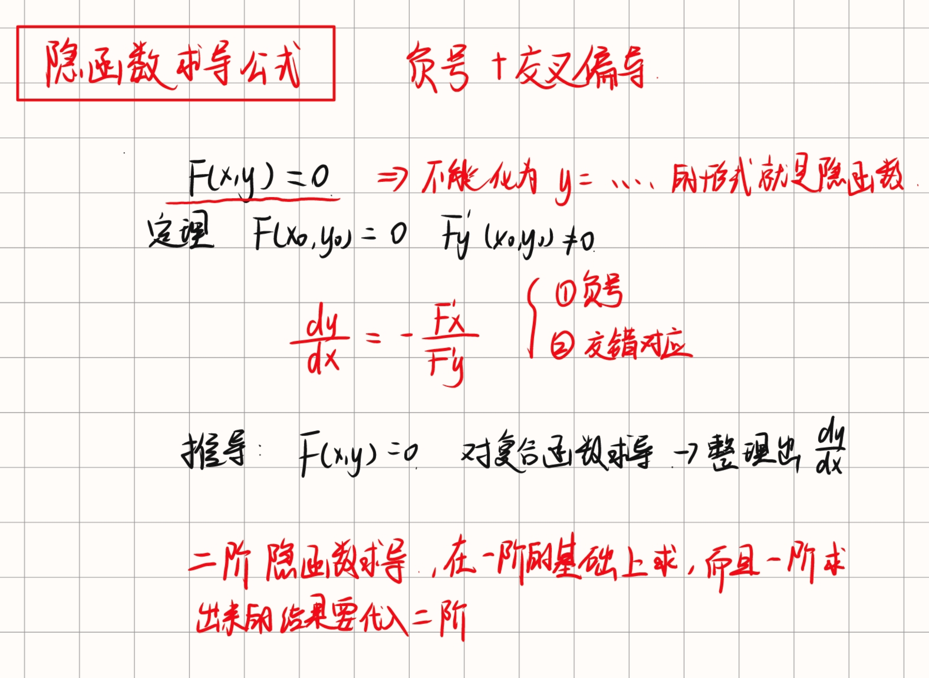
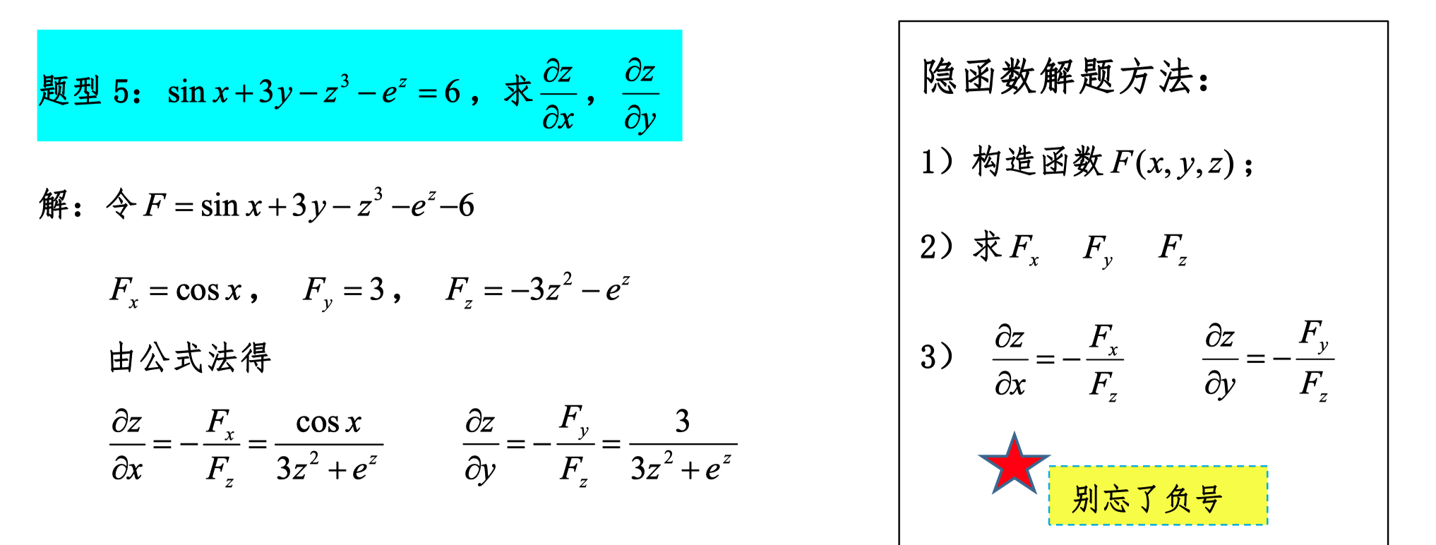
Partial Derivatives of Implicit Functions

Higher-Order Partial Derivatives

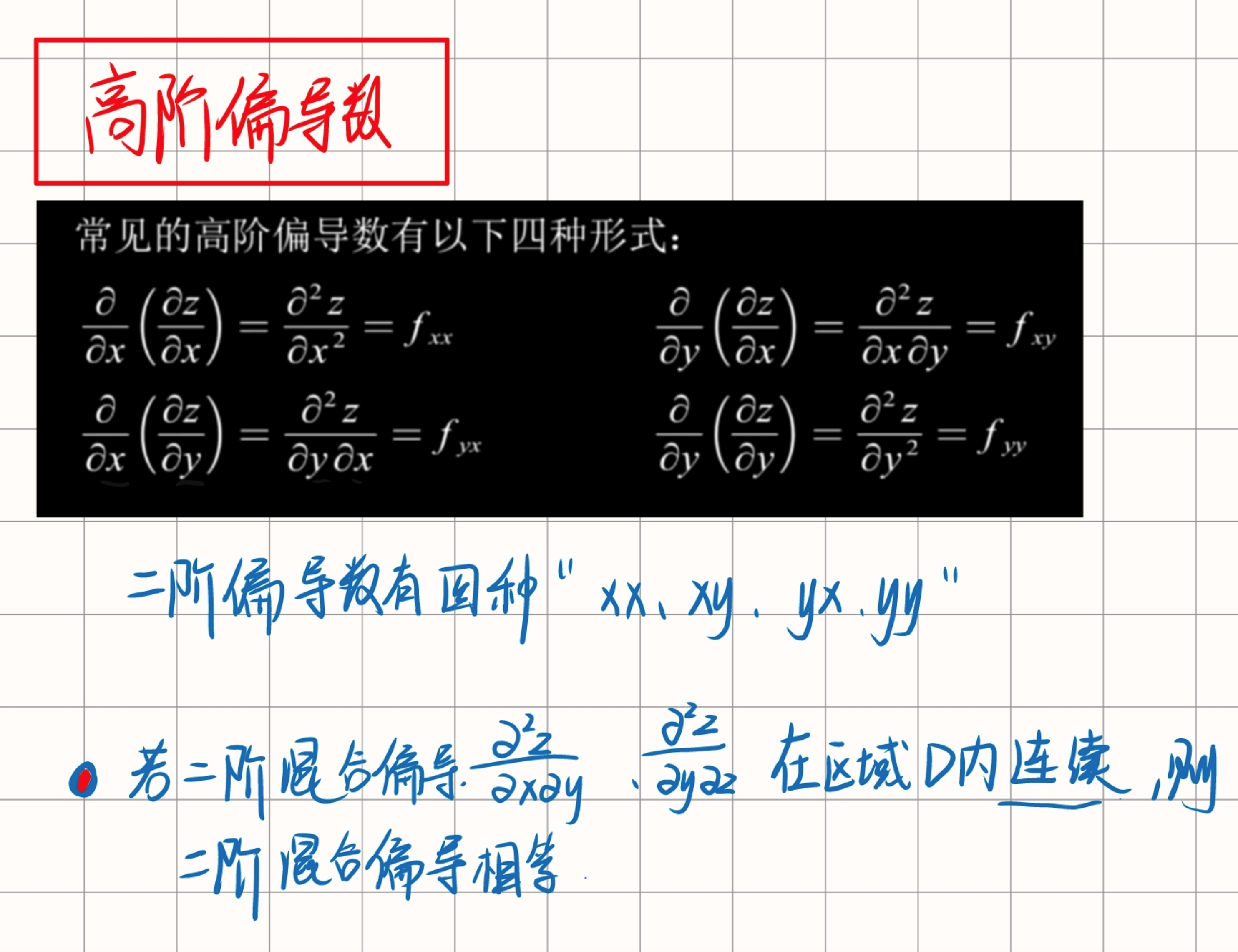
"f has continuous second-order partial derivatives" means mixed partial derivatives are equal.

This means that all second-order partial derivatives of function f exist and are continuous. Specifically, if we have a function f whose partial derivatives can be written as f_x, f_y, etc., then its second-order partial derivatives can be written as f_xx, f_yy, f_xy, f_yx, etc. For function f, having continuous second-order partial derivatives means:

1. All these second-order partial derivatives exist.
2. These second-order partial derivatives are continuous functions.
3. Mixed partial derivatives are equal, i.e., f_xy = f_yx.

To understand this concept, consider a specific example. Suppose we have a function f(x, y), and we compute its first and second-order partial derivatives:

• First-order partial derivatives:

  $$f_x = \frac{\partial f}{\partial x}, \quad f_y = \frac{\partial f}{\partial y}$$

• Second-order partial derivatives:

  $$f_{xx} = \frac{\partial^2 f}{\partial x^2}, \quad f_{yy} = \frac{\partial^2 f}{\partial y^2}, \quad f_{xy} = \frac{\partial^2 f}{\partial x \partial y}, \quad f_{yx} = \frac{\partial^2 f}{\partial y \partial x}$$

If f has continuous second-order partial derivatives, then we can guarantee f_xy = f_yx. This is according to Clairaut's Theorem or Schwarz's Theorem, which states that if the mixed partial derivatives of f exist and are continuous, then they are equal.

For this specific problem, assuming z = f(xy, x/y) + sin y, and f has continuous second-order partial derivatives, this means we can use f₁₂ = f₂₁ when computing the mixed second-order partial derivative ∂²z/∂x∂y. This mathematically provides us with a tool for simplifying calculations, because we know these mixed partial derivatives will be equal during computation.

In summary, the property of "having continuous second-order partial derivatives" ensures that during partial derivative calculations, we can rely on the symmetry of mixed partial derivatives, thereby simplifying the computation process. This is an important concept in multivariable calculus.

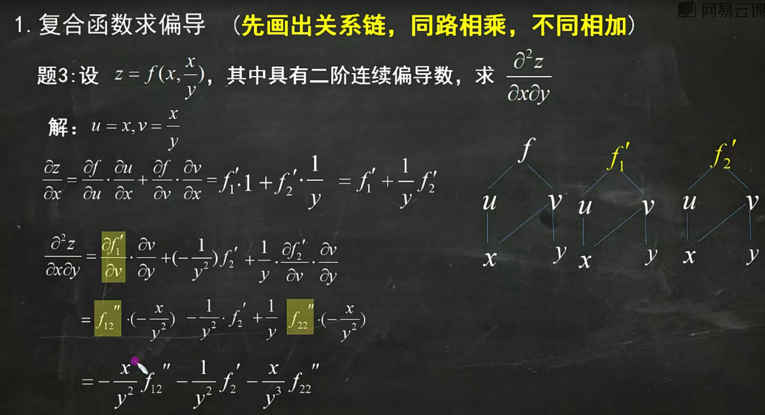
Partial Derivatives of Composite Functions

First draw the relationship chain: same path means multiply, different paths means add.

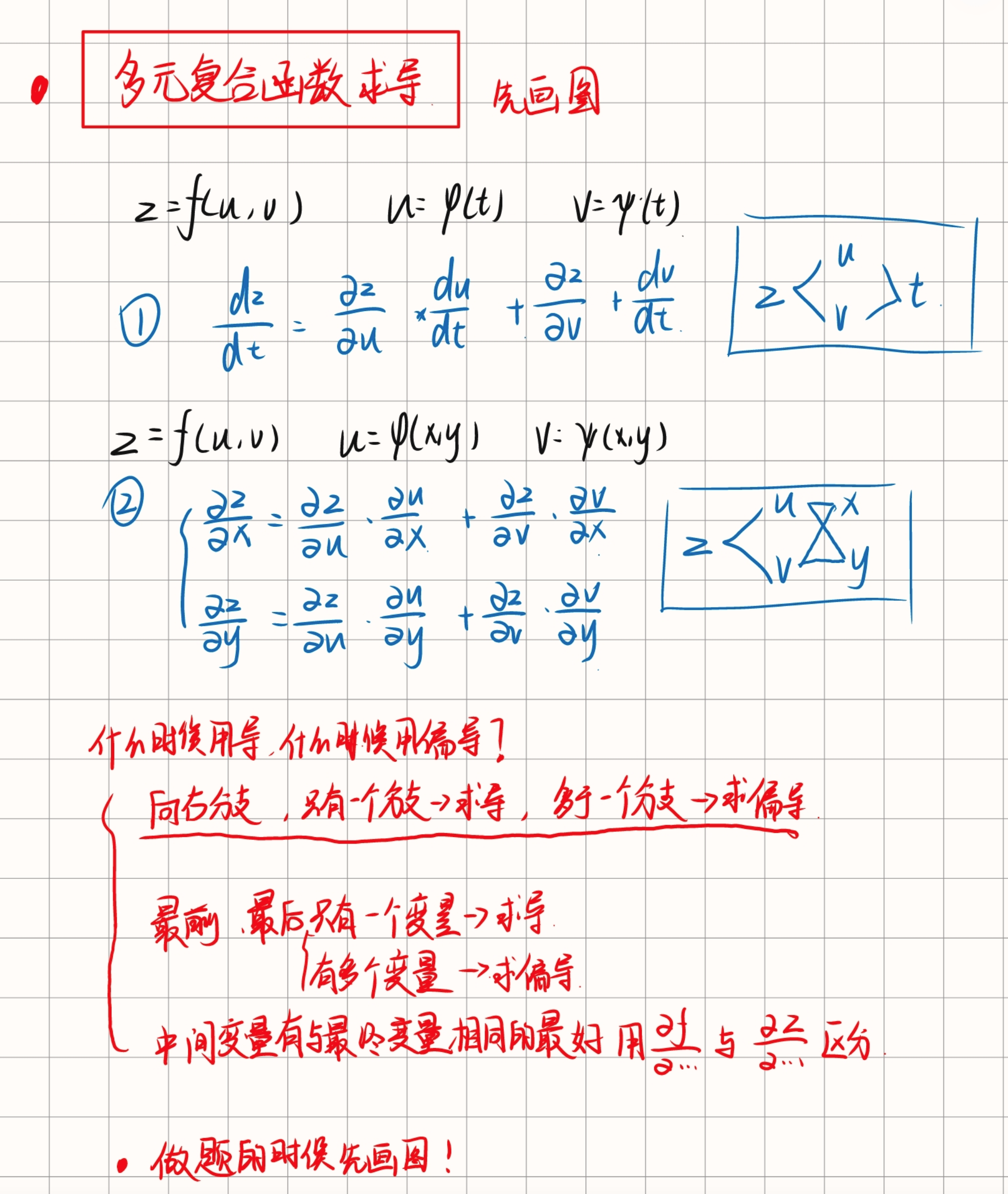
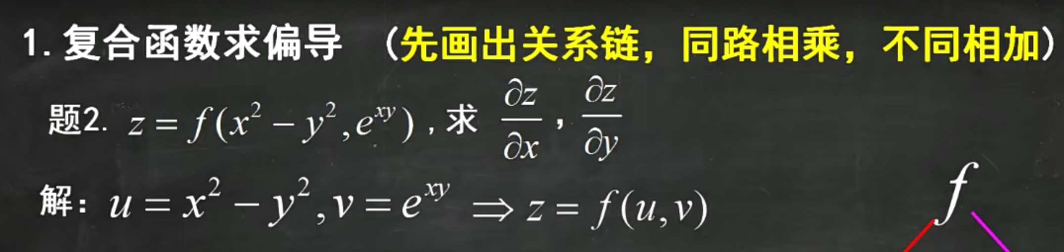
When encountering expressions written inside, first use parameters to substitute them out before proceeding.

After taking partial derivatives, the relationship chain remains the same as the original function.

When computing second-order partial derivatives of composite functions, pay attention to the "first leads, second doesn't" type of composite function.

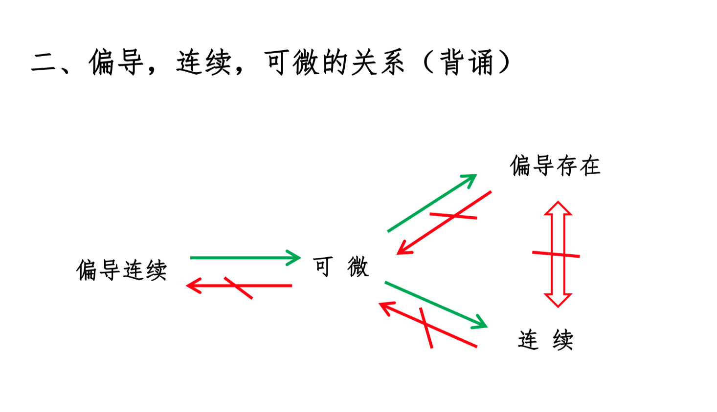
Relationships Among Partial Derivatives, Continuity, and Differentiability

Note

Here, "continuous partial derivatives" means the function's partial derivatives exist and the partial derivatives are continuous at that point.

Here, "continuous" means the function is continuous at that point.

Here, "partial derivatives exist" means the function's partial derivatives exist at that point.

1. Differentiable ⇒ Partial Derivatives Exist (Necessary Condition)

Assume a function f(x, y) is differentiable at a point (a, b). This means there exists a linear approximation:

$$f(a + h, b + k) = f(a, b) + f_x(a, b) h + f_y(a, b) k + o(\sqrt{h^2 + k^2})$$

where f_x(a, b) and f_y(a, b) are the partial derivatives of f at point (a, b). Because differentiability means the function near a point can be approximated by a linear function, the partial derivatives must exist. This is a necessary condition for differentiability.

2. Partial Derivatives Exist ⇏ Differentiable (Existence of Partial Derivatives Does Not Imply Differentiability)

Even if all partial derivatives of a function exist at a point, the function may not be differentiable at that point. For example, consider the function

$$f(x, y) = \begin{cases} \frac{x^2 y}{x^2 + y^2}, & (x, y) \neq (0, 0) \\ 0, & (x, y) = (0, 0) \end{cases}$$

We can compute the partial derivatives at the origin: f_x(0, 0) = 0 and f_y(0, 0) = 0, but the function is not differentiable at the origin because its increment cannot be well approximated by a linear function.

3. Differentiable ⇒ Continuous (Sufficient Condition)

If a function is differentiable at a point, then it is certainly continuous at that point. Differentiability means that not only does a good linear approximation exist at that point, but the function value also changes with small changes in the variables. If a function is differentiable at a point, the function values near that point approach the function value at that point, meaning the function is continuous at that point.

4. Continuous ⇏ Differentiable (Continuity Does Not Imply Differentiability)

Even if a function is continuous at a point, it may not be differentiable at that point. For example, the absolute value function f(x) = |x| is continuous at x = 0, but not differentiable at that point because the left and right derivatives are not equal.

5. Partial Derivatives Exist and Are Continuous ⇒ Differentiable (Sufficient Condition)

If a function's partial derivatives exist and are continuous at a point, then the function is differentiable at that point. For example, for a function f(x, y), if f_x and f_y both exist and are continuous at point (a, b), then f is differentiable at that point. This is a sufficient condition.

Through these relationships, we can better understand the connections between differentiability, continuity, and the existence of partial derivatives. In practical applications, these concepts are very important for function analysis and research.

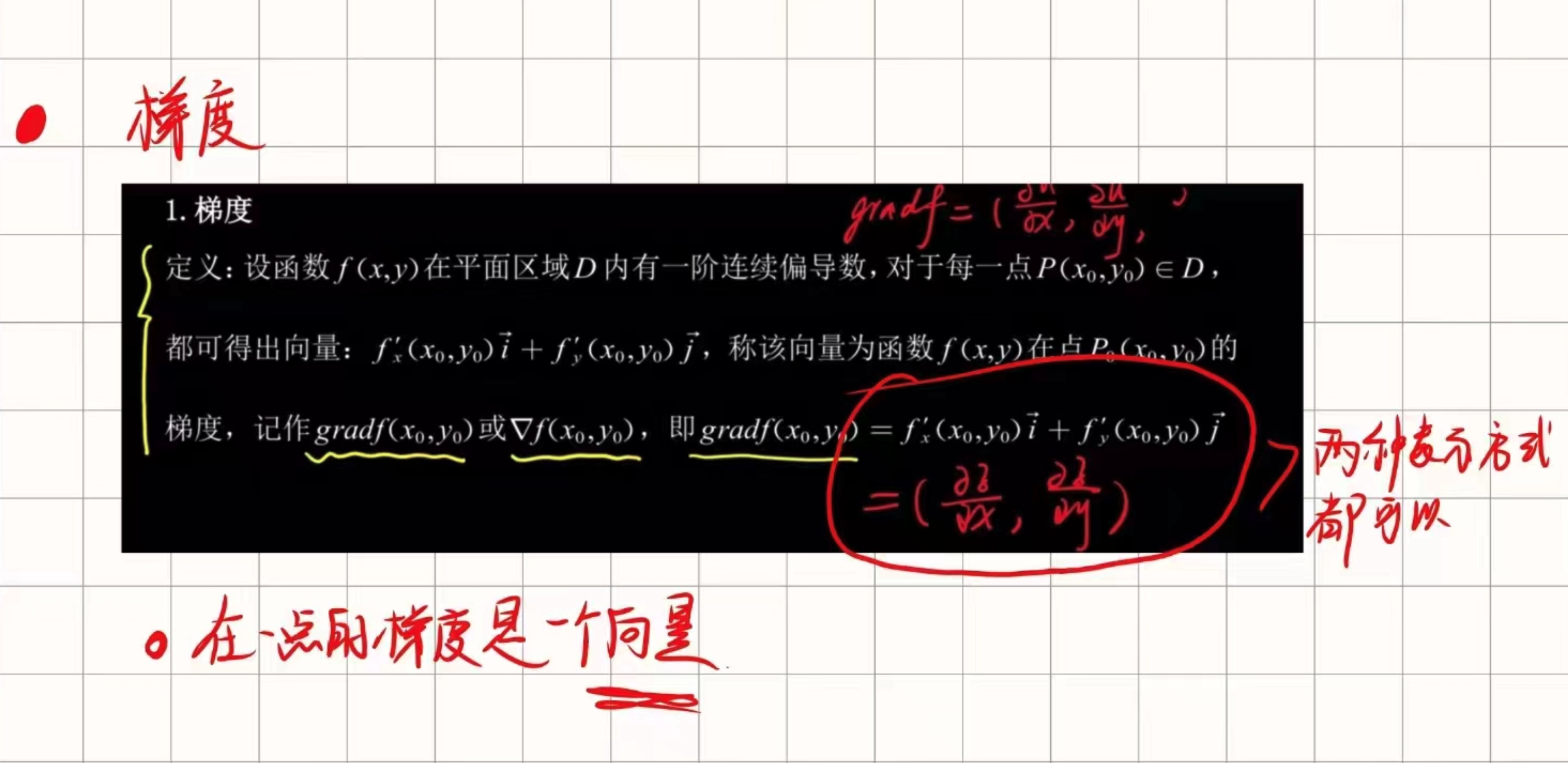
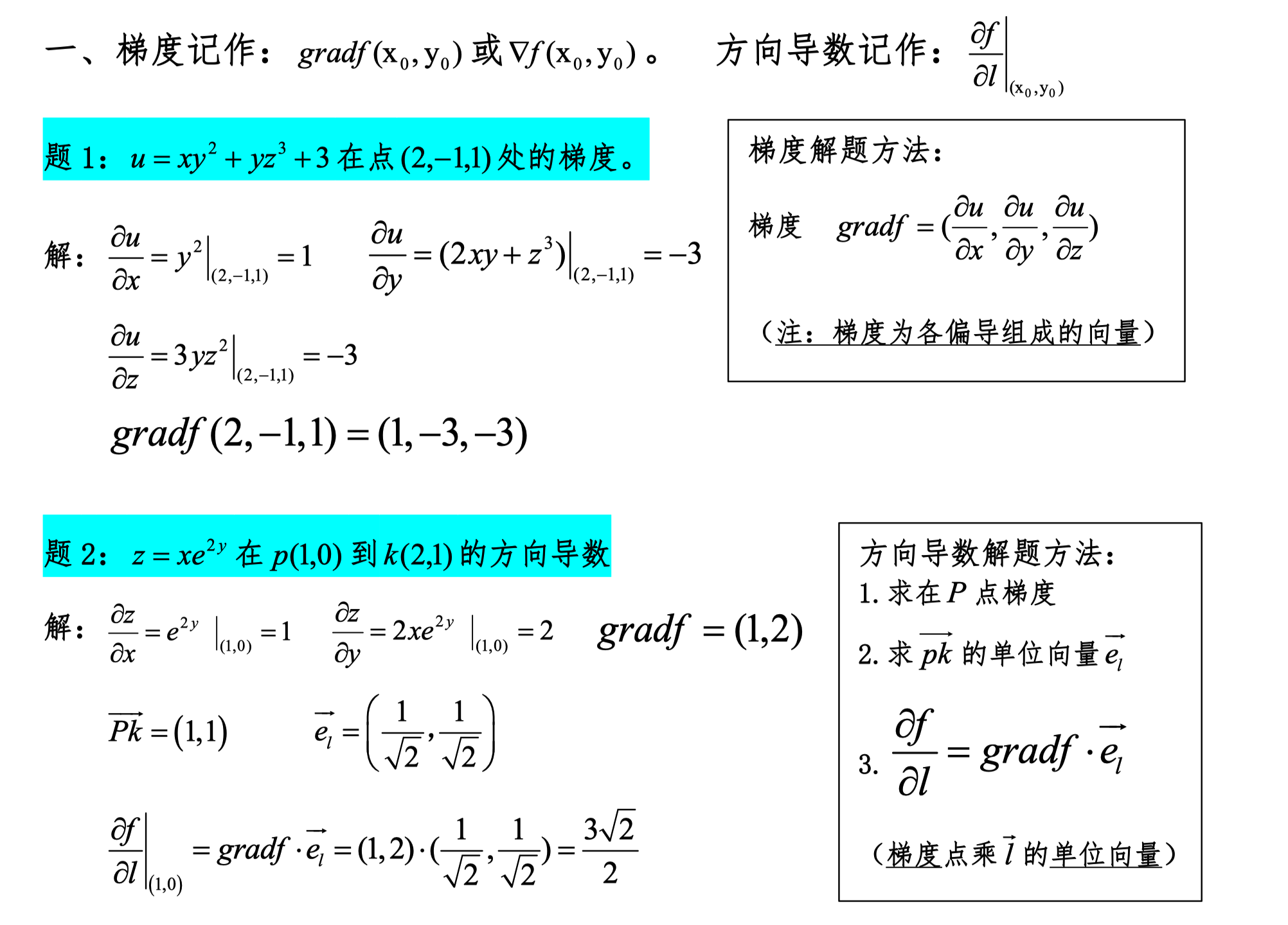
Gradient, Directional Derivative

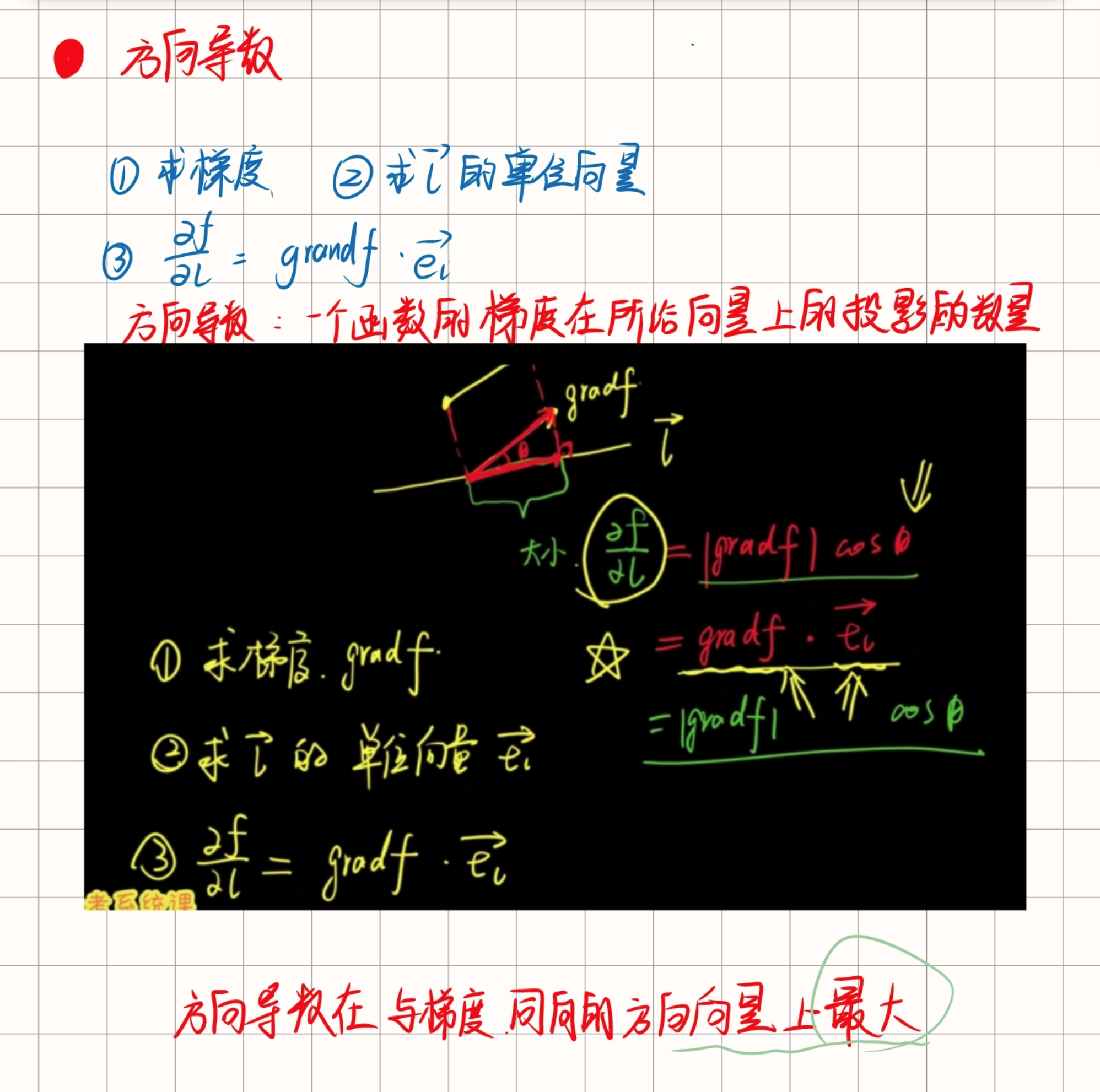
The maximum value of the directional derivative equals the magnitude of the gradient.

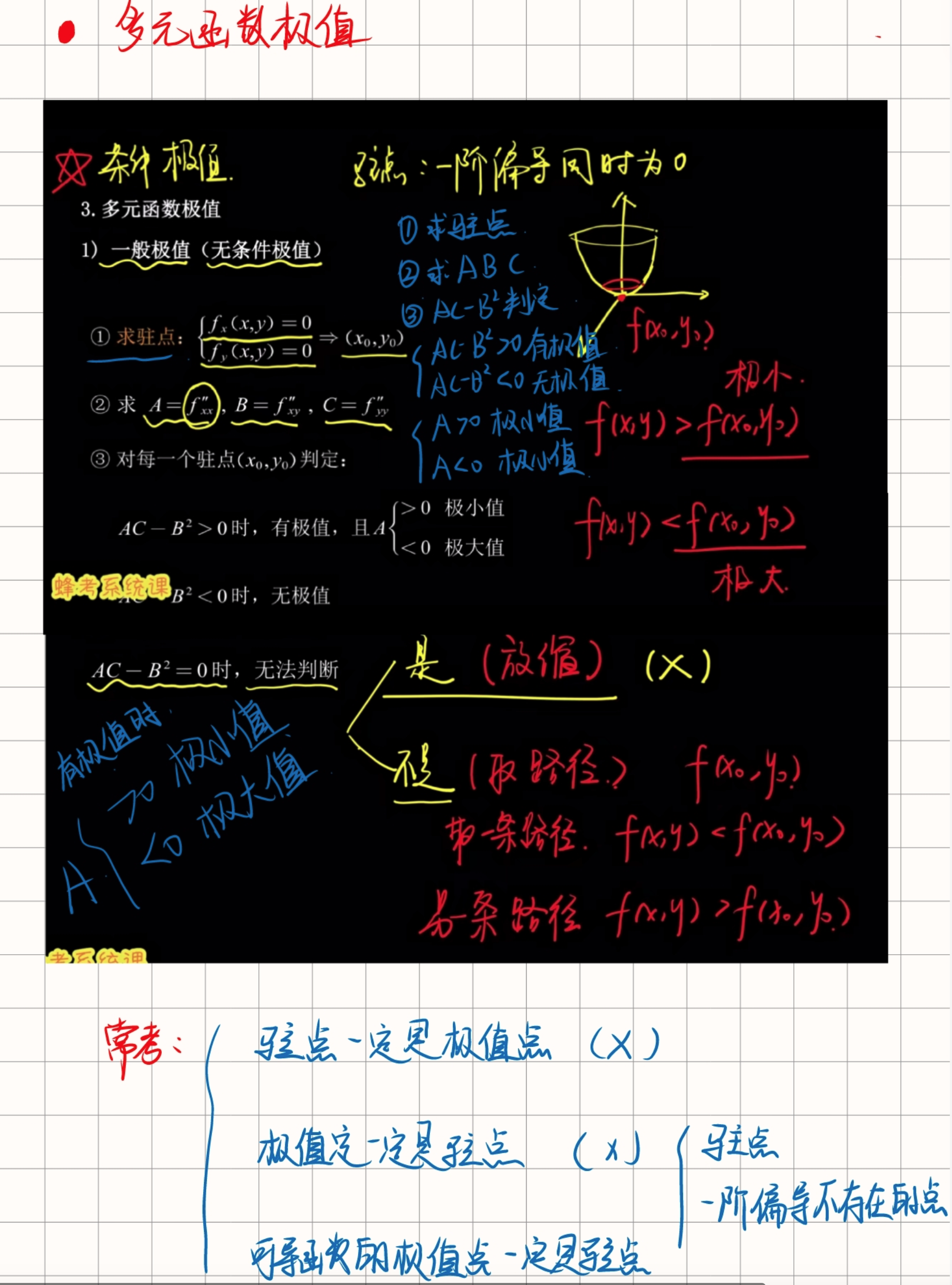
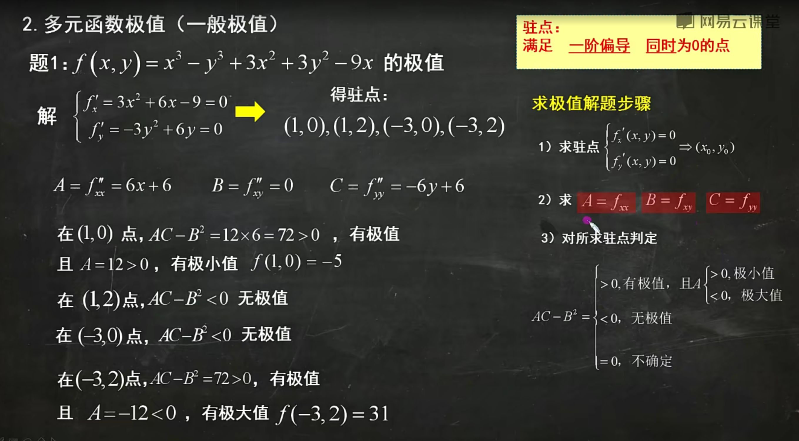
Extrema of Multivariable Functions

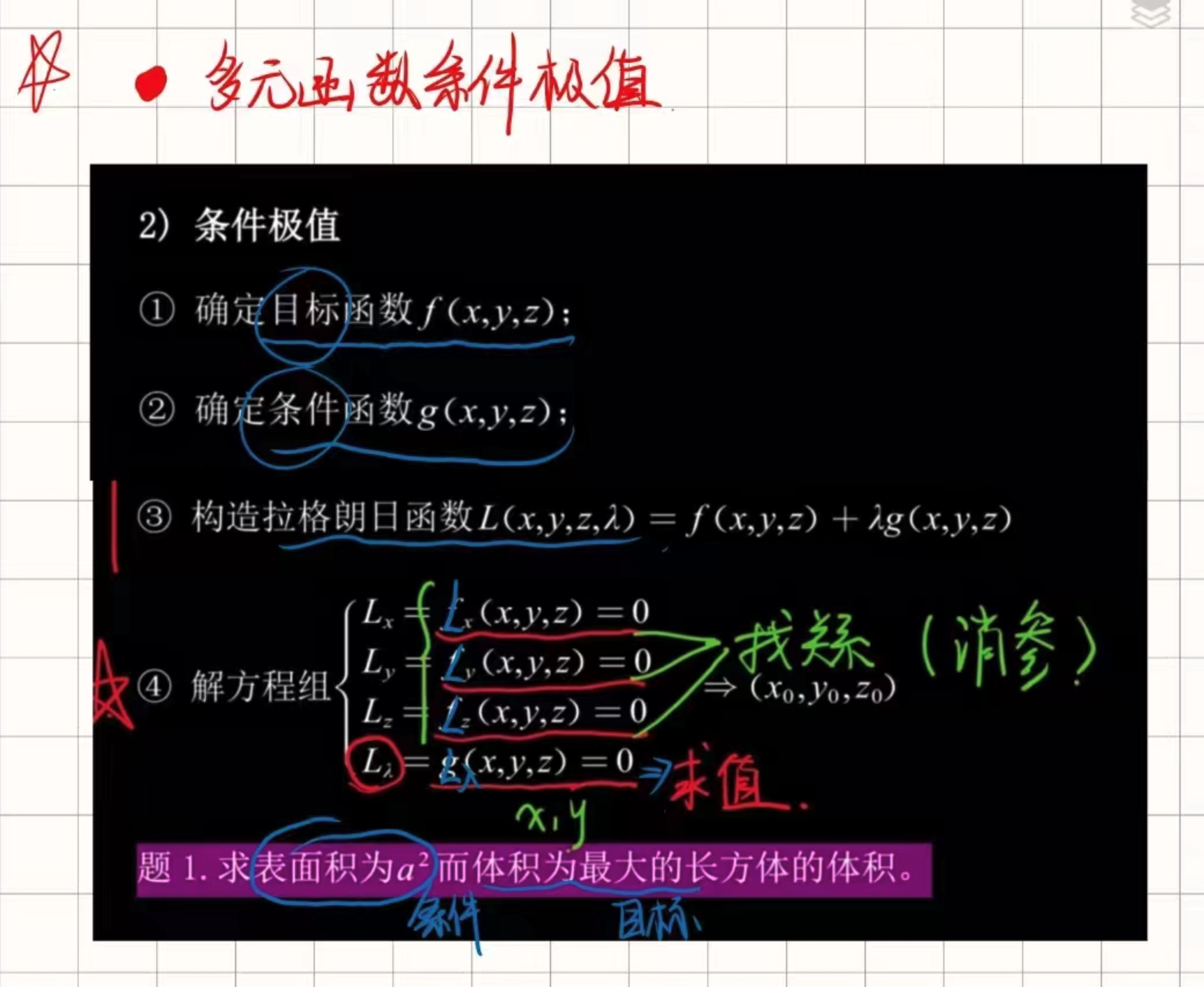
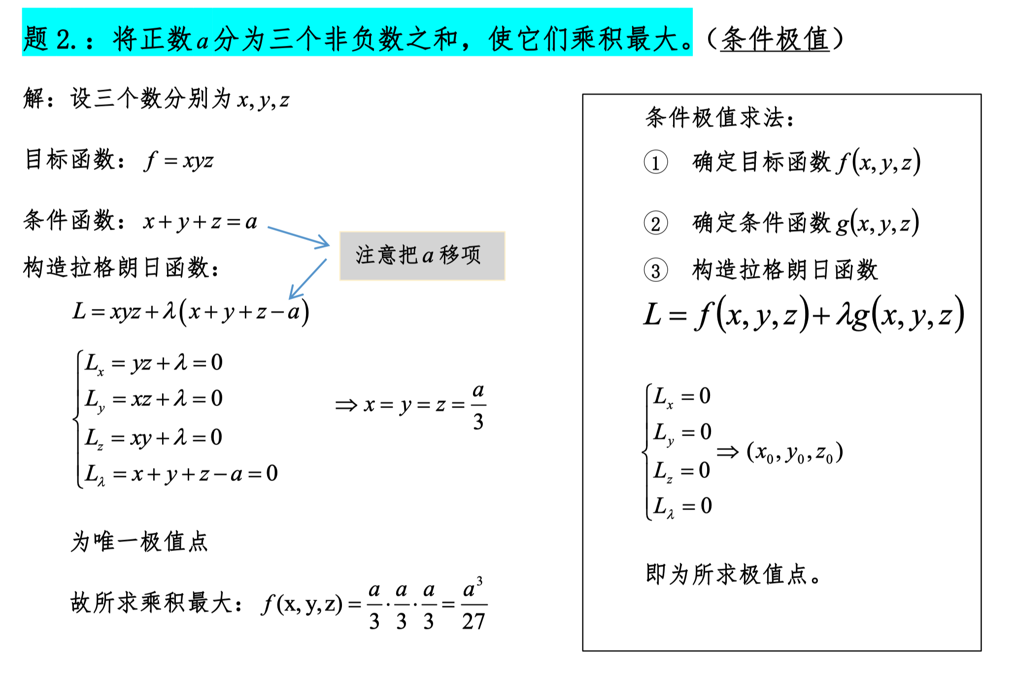
Conditional Extrema of Multivariable Functions

Space Geometry

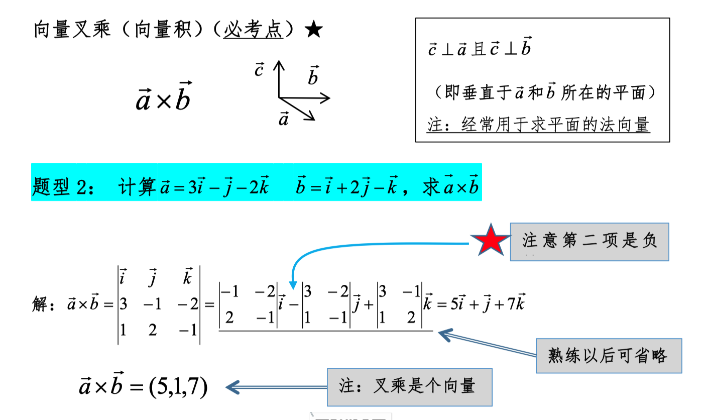
Cross Product

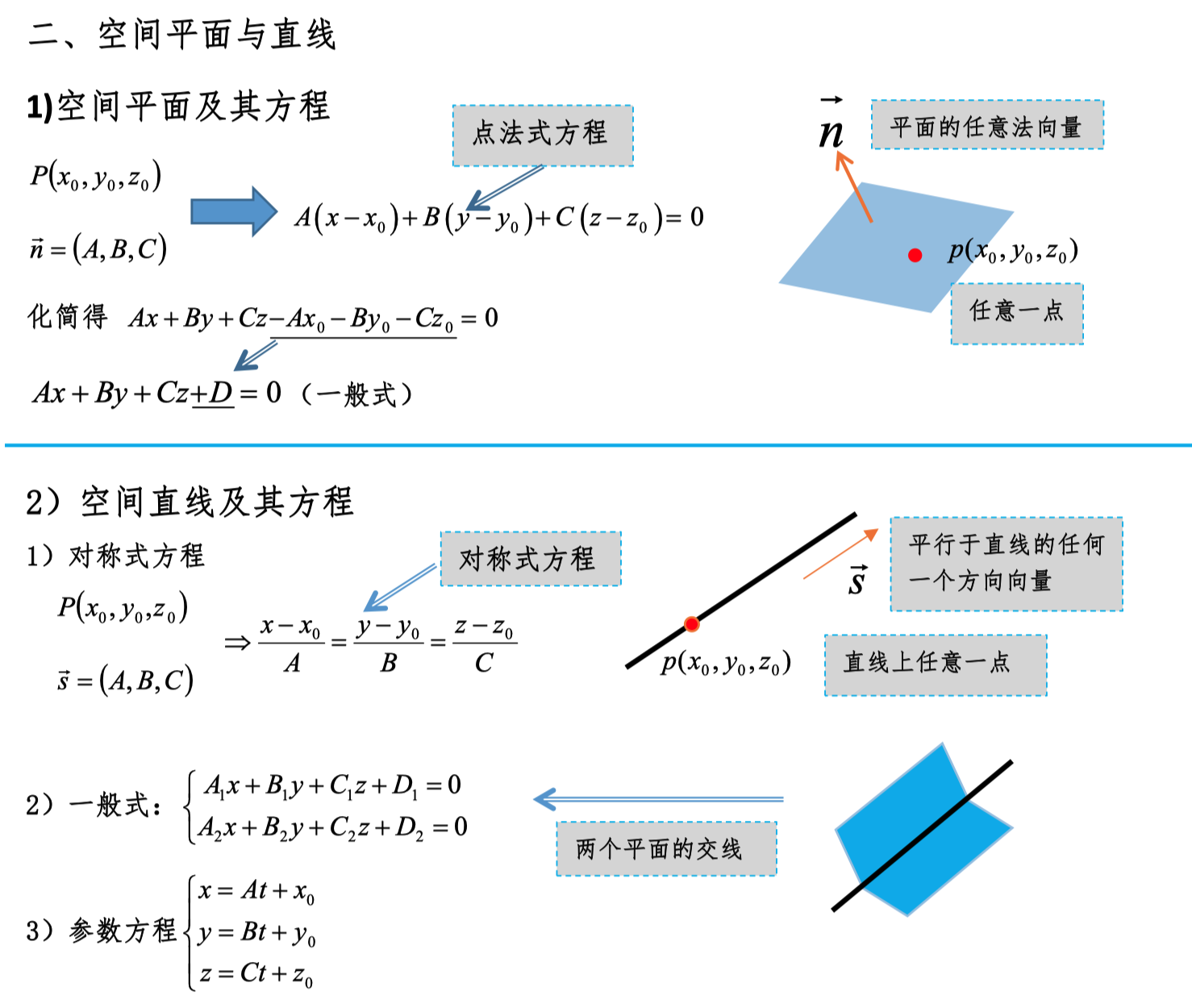
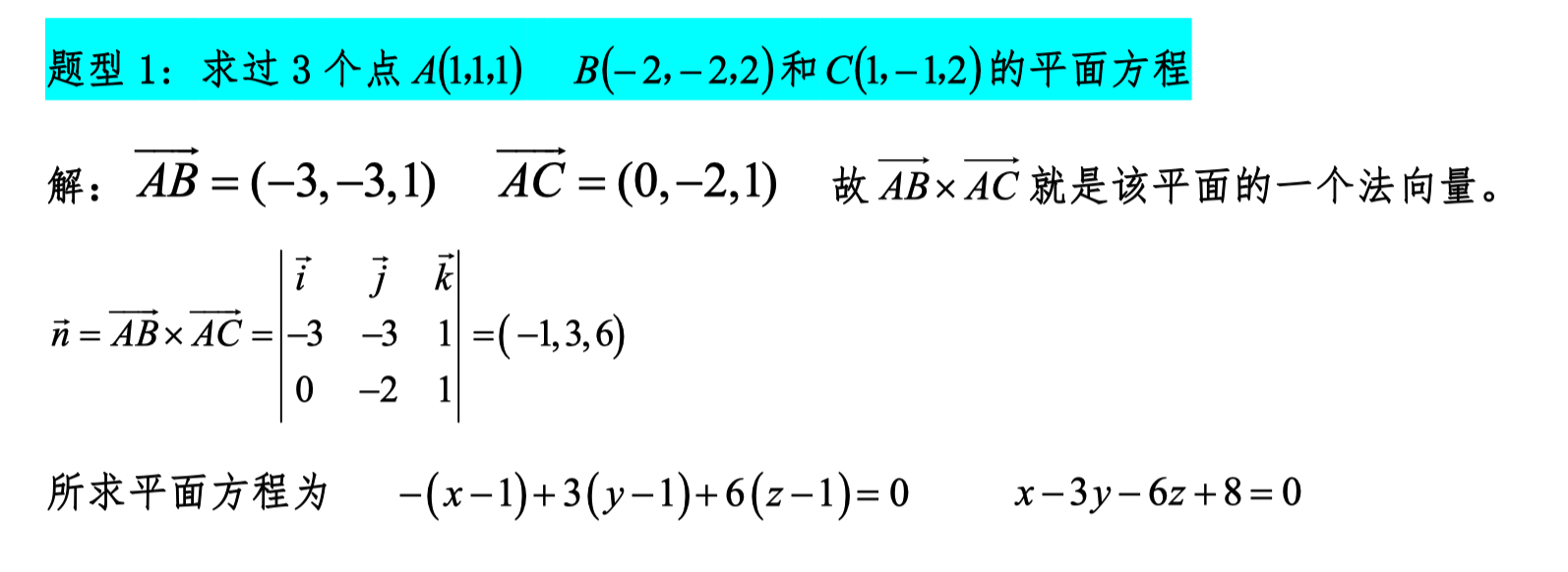
Lines and Planes

Finding Symmetric Equations

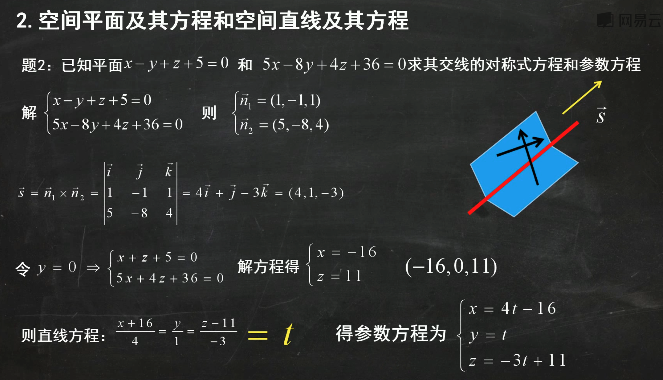
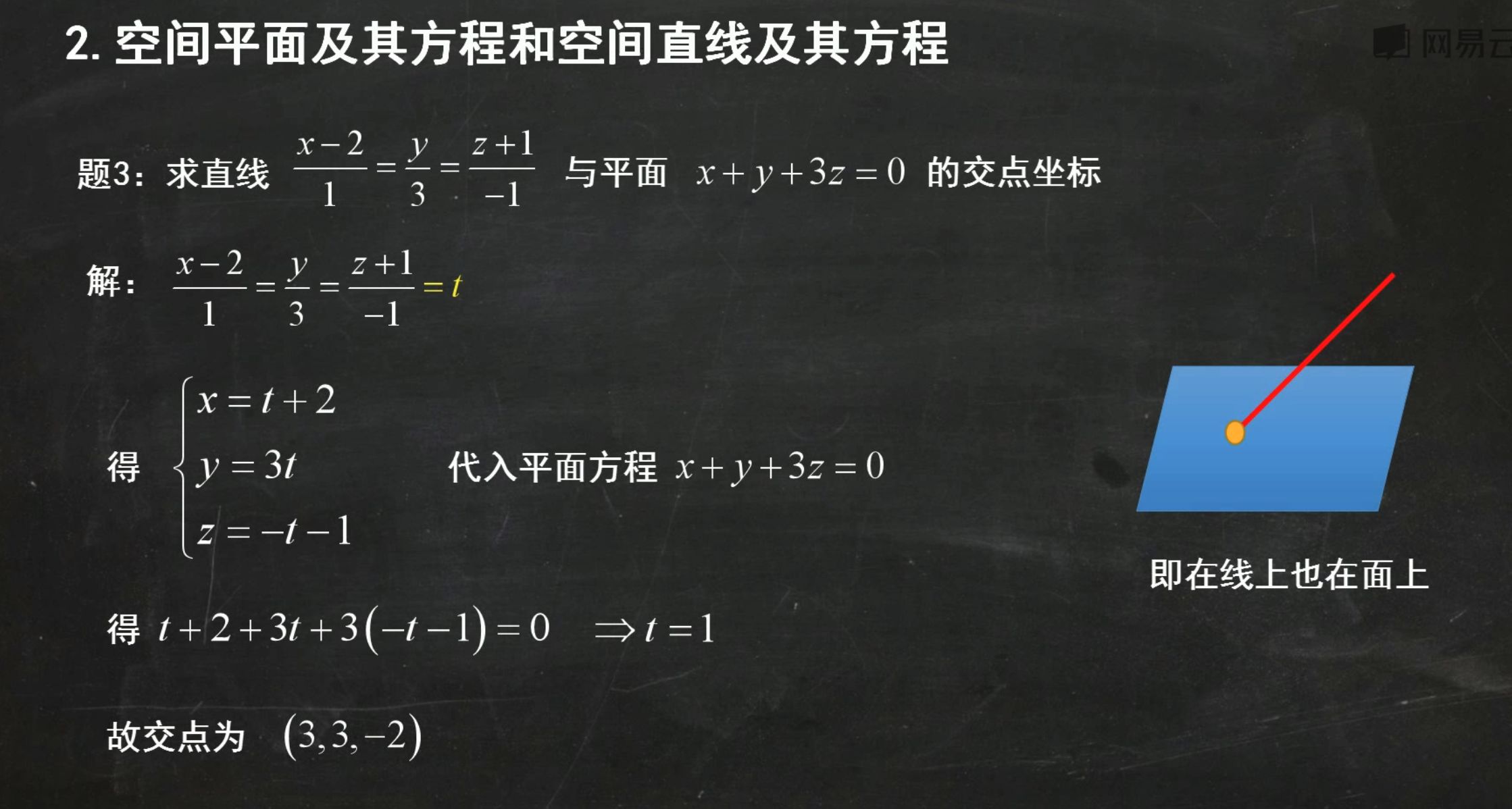
Using Parametric Equations to Find Intersection Coordinates

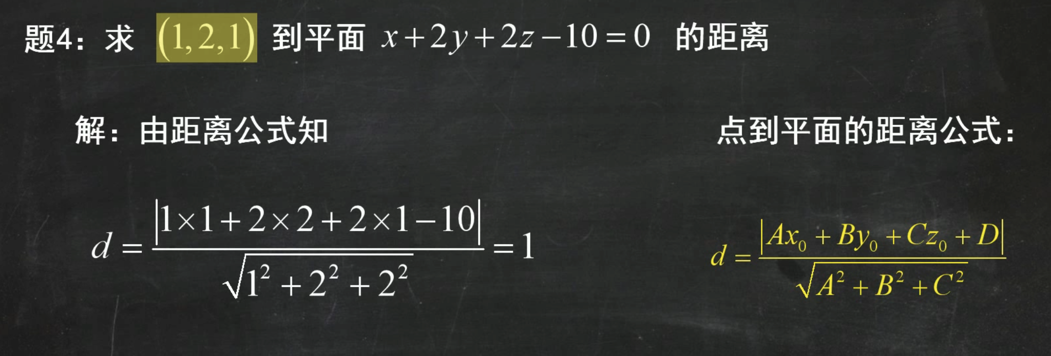
Distance Formula from a Point to a Plane

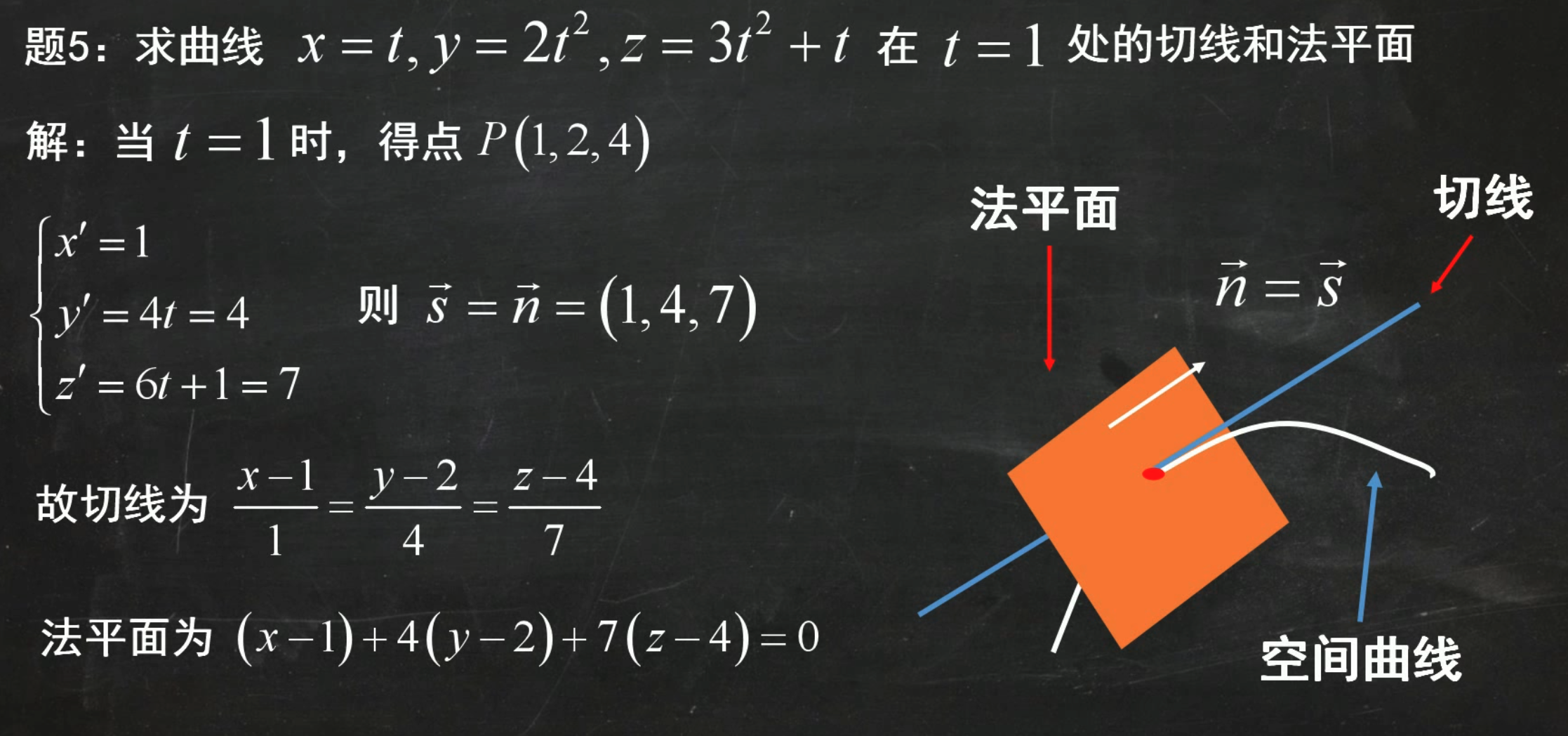
Tangent Lines and Normal Planes

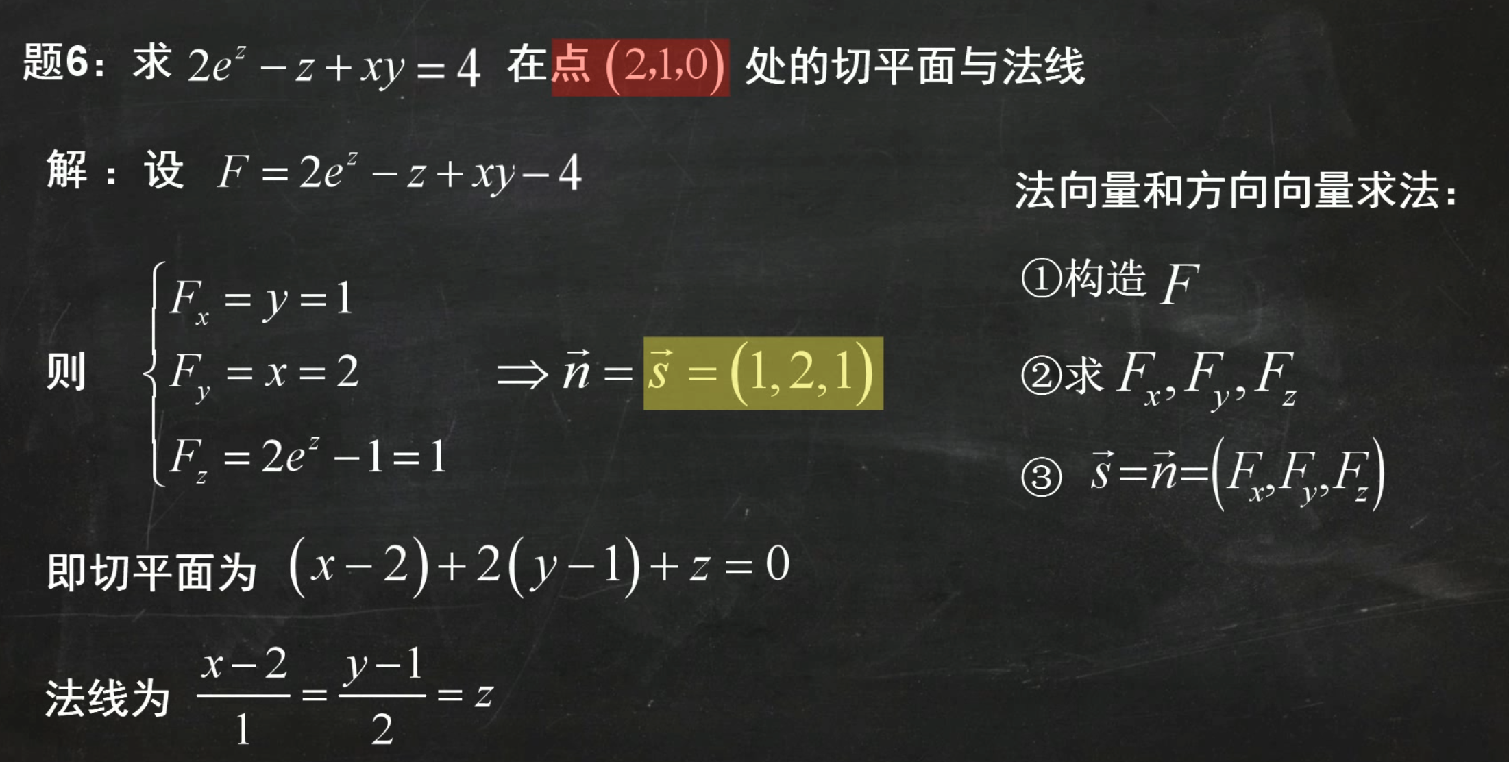
Tangent Planes and Normal Lines

Gradient of Curves, Gradient of Surfaces

Yes, your understanding is correct. Specifically:

1. Gradient of a curve: For a space curve, the gradient vector at a point can be regarded as the direction vector of the tangent line at that point.

2. Gradient of a surface: For a surface, the gradient vector (i.e., the normal vector) at a point is indeed the normal vector of the tangent plane at that point.

Explanation

Gradient vector of a curve: Suppose a curve is described by the parametric equation r(t) = (x(t), y(t), z(t)). The direction vector of the tangent line at a point P on the curve is the derivative vector r'(t) at that point.

Gradient vector of a surface: Suppose a surface is described by the implicit function F(x, y, z) = 0. The gradient vector ∇F = (∂F/∂x, ∂F/∂y, ∂F/∂z) at a point P on the surface is the normal vector of the tangent plane at that point. The equation of the tangent plane can be written as:

$$\nabla F \cdot \mathbf{r} = \nabla F \cdot \mathbf{r_0}$$

where r is the position vector of any point on the plane, and r₀ is the position vector of point P on the surface.

In summary:

• The direction vector of the tangent line at a point on a curve can be obtained by finding the derivative vector at that point.
• The normal vector of the tangent plane at a point on a surface is the gradient vector at that point.

Gradient of Surfaces in Explicit Function Form

Suppose a surface is expressed in explicit function form, for example z = f(x, y). We can still find the gradient vector, which is the normal vector of the tangent plane at that point.

1. Find Partial Derivatives

• Compute the partial derivative of f with respect to x, denoted ∂f/∂x.
• Compute the partial derivative of f with respect to y, denoted ∂f/∂y.

2. Construct the Gradient Vector

For a surface in explicit function form z = f(x, y), at point P(x₀, y₀, z₀), the gradient vector ∇f is: $( \nabla f = \left( \frac{\partial f}{\partial x}, \frac{\partial f}{\partial y}, -1 \right) )$

3. Verify the Gradient Vector Is the Normal Vector

The gradient vector ∇f obtained from the above calculation is the normal vector of the tangent plane at that point.

Example

Let the surface be z = x² + y². Find the gradient vector at point P(1, 1, 2):

1. Find partial derivatives: $( \frac{\partial z}{\partial x} = 2x \quad \text{and} \quad \frac{\partial z}{\partial y} = 2y )$

2. Compute the gradient vector at point P(1, 1, 2): $( \left( \frac{\partial z}{\partial x}, \frac{\partial z}{\partial y}, -1 \right) = \left( 2 \cdot 1, 2 \cdot 1, -1 \right) = (2, 2, -1) )$

3. Verify the gradient vector: The gradient vector (2, 2, -1) is the normal vector of the tangent plane to the surface z = x² + y² at point P(1, 1, 2).

Tangent Plane Equation

The tangent plane equation expressed in point-normal form is: $( 2(x - 1) + 2(y - 1) - 1(z - 2) = 0 )$

Simplifying: $( 2x + 2y - z = 4 )$

In summary, for surfaces in explicit function form, we can find the gradient vector by computing partial derivatives, and this gradient vector is the normal vector of the tangent plane.

Double Integrals

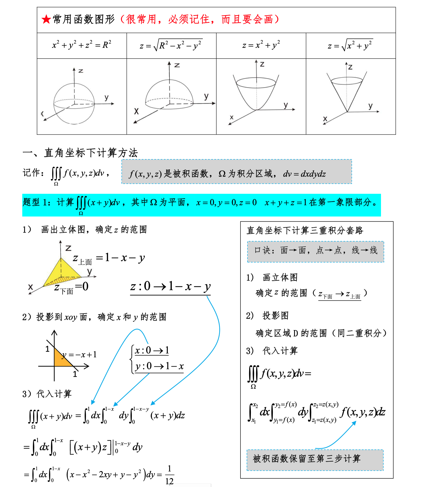
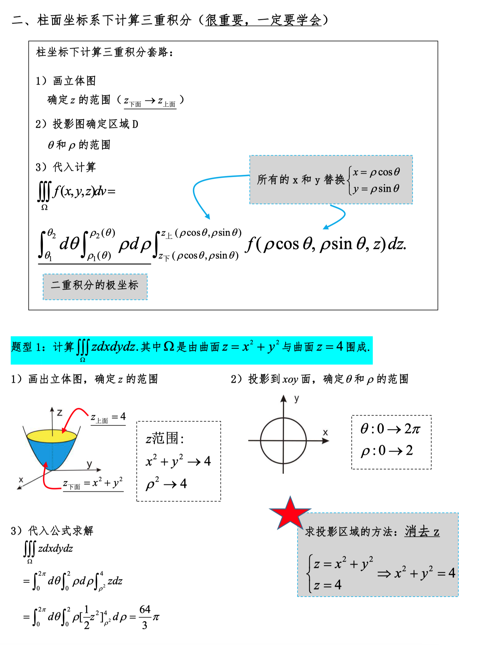
Triple Integrals

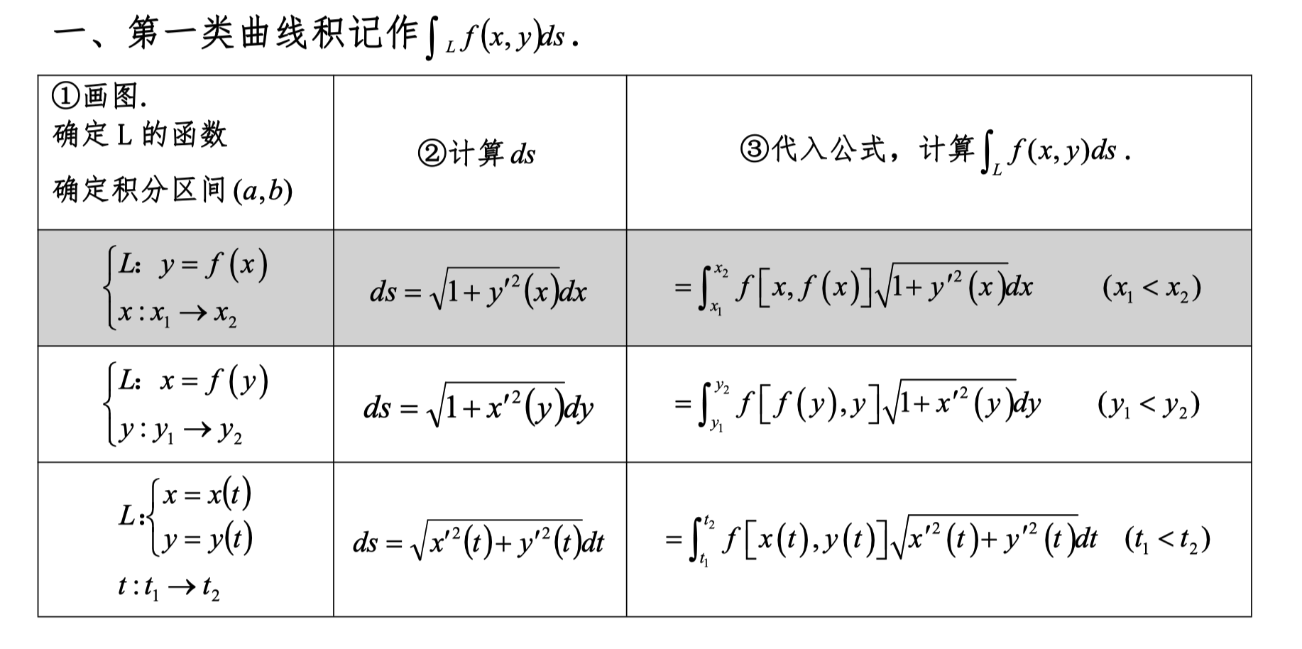
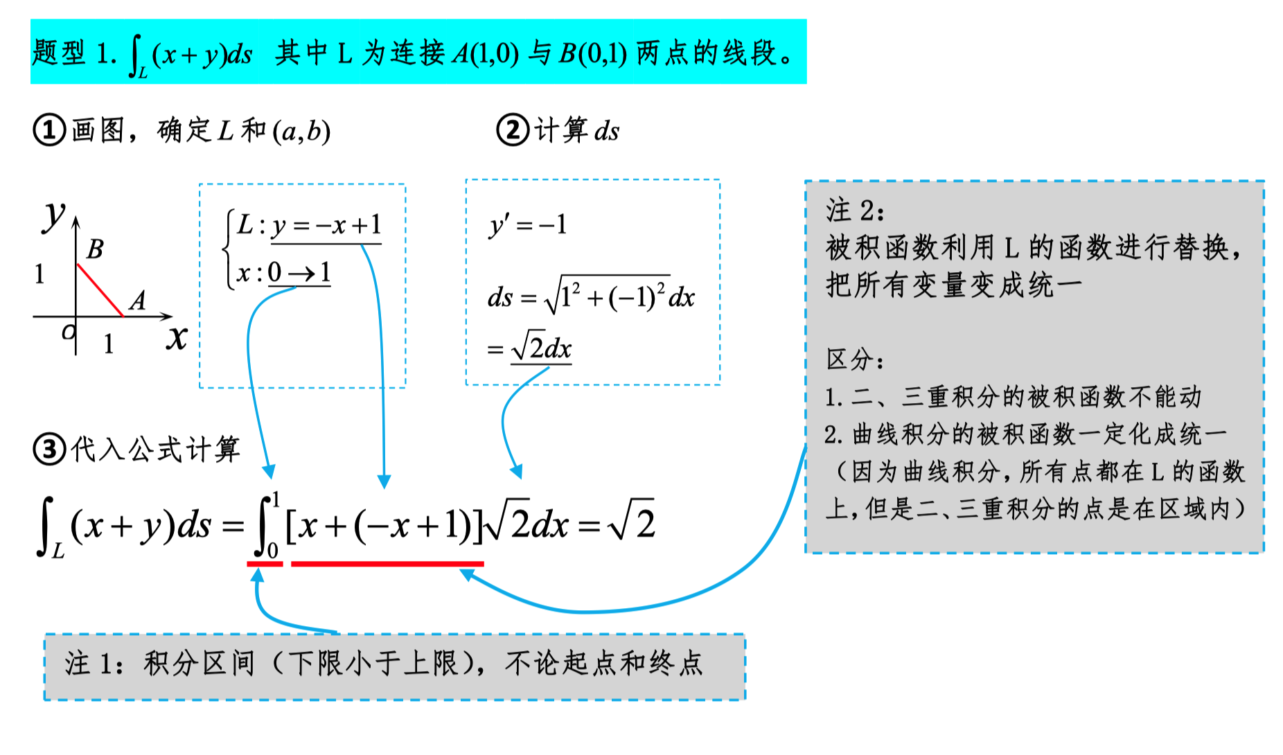
Line Integrals of the First Kind

Note

Here, the range of x is only about magnitude: from small to large, regardless of starting and ending points.

In line integrals of the second kind, only the starting and ending points matter, not the magnitude.

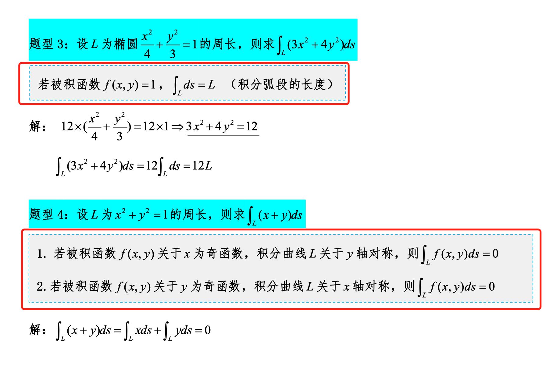
Before solving, first check if the integral curve is symmetric about any axis.

The geometric meaning of the line integral of the first kind mainly involves the cumulative effect of a scalar field function along a curve. Specifically, it reflects the total accumulation of the scalar field along the curve. Let curve C be a smooth curve in a plane or space, and let the scalar field function f be defined on curve C. The geometric meaning of the line integral of the first kind ∫_C f ds can be explained as follows:

Geometric Meaning

• Cumulative quantity along the curve: The line integral of the first kind represents the sum of the scalar field f at each point on curve C multiplied by the curve length element ds at that point. Therefore, it reflects the cumulative effect of function f along curve C.
• Weighted length: If the scalar field f represents some density (such as mass density, energy density, etc.), then ∫_C f ds represents the weighted length along curve C, i.e., the sum of the density at each point multiplied by the corresponding small segment length.

Mathematical Expression

Let curve C be described by the parametric equation r(t), where t varies in the interval [a, b]. The line integral of the first kind can be expressed as:

$$\int_C f \, ds = \int_a^b f(\mathbf{r}(t)) \|\mathbf{r}'(t)\| \, dt$$

where r(t) is the parametric equation of the curve, r'(t) is its derivative, and ‖r'(t)‖ represents the magnitude of the derivative, i.e., the speed of the curve at t.

Example

Suppose there is a curve C on a plane defined as y = x², from point (0, 0) to (1, 1), with function f(x, y) = x + y. The line integral of the first kind represents the cumulative effect of f(x, y) along the curve y = x².

We can parameterize the curve as r(t) = (t, t²), where t varies in [0, 1]. Then,

$$\int_C (x + y) \, ds = \int_0^1 (t + t^2) \sqrt{1 + (2t)^2} \, dt$$

This integral represents the total accumulation of function f(x, y) along the curve y = x² from (0, 0) to (1, 1).

In summary, the geometric meaning of the line integral of the first kind is mainly that it describes the cumulative effect of a scalar field function along a specific curve, reflecting the sum of the scalar field value at each point on the curve multiplied by the curve length element.

A Simple Example

Suppose you are walking along a river, and the depth of the river keeps changing. You want to know the total volume of water in the river. You can multiply the length of each small segment of the river by the depth of that segment, then sum up the results of all segments. This is the basic idea of the line integral of the first kind.

Expressed as a formula, suppose the curve is C and the function is f, then the line integral of the first kind ∫_C f ds can be understood as:

$$\int_C f \, ds = \text{value (depth) of each small segment} \times \text{length of that segment}$$

Then, summing up the results of all segments gives the total value.

Line Integrals of the Second Kind

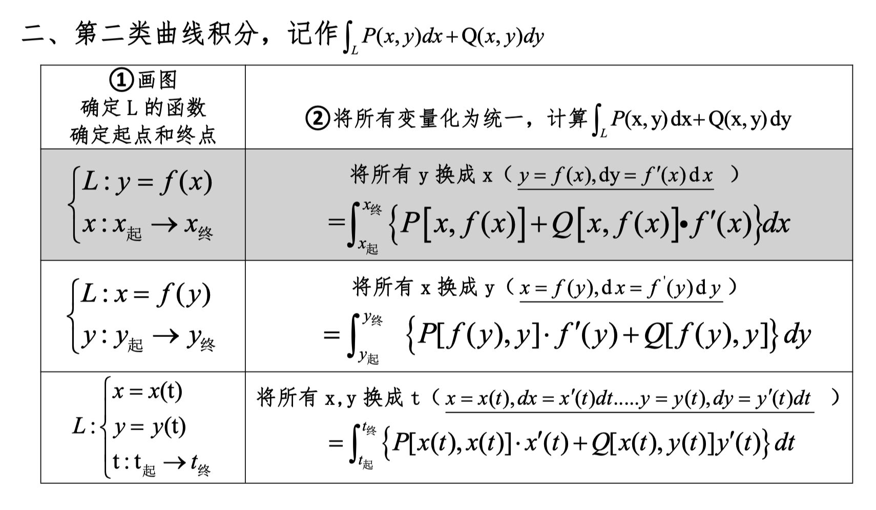
Note

In line integrals of the second kind, only the starting and ending points matter, not the magnitude.

Green's Theorem

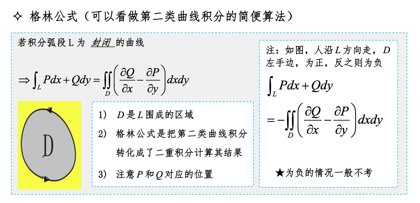
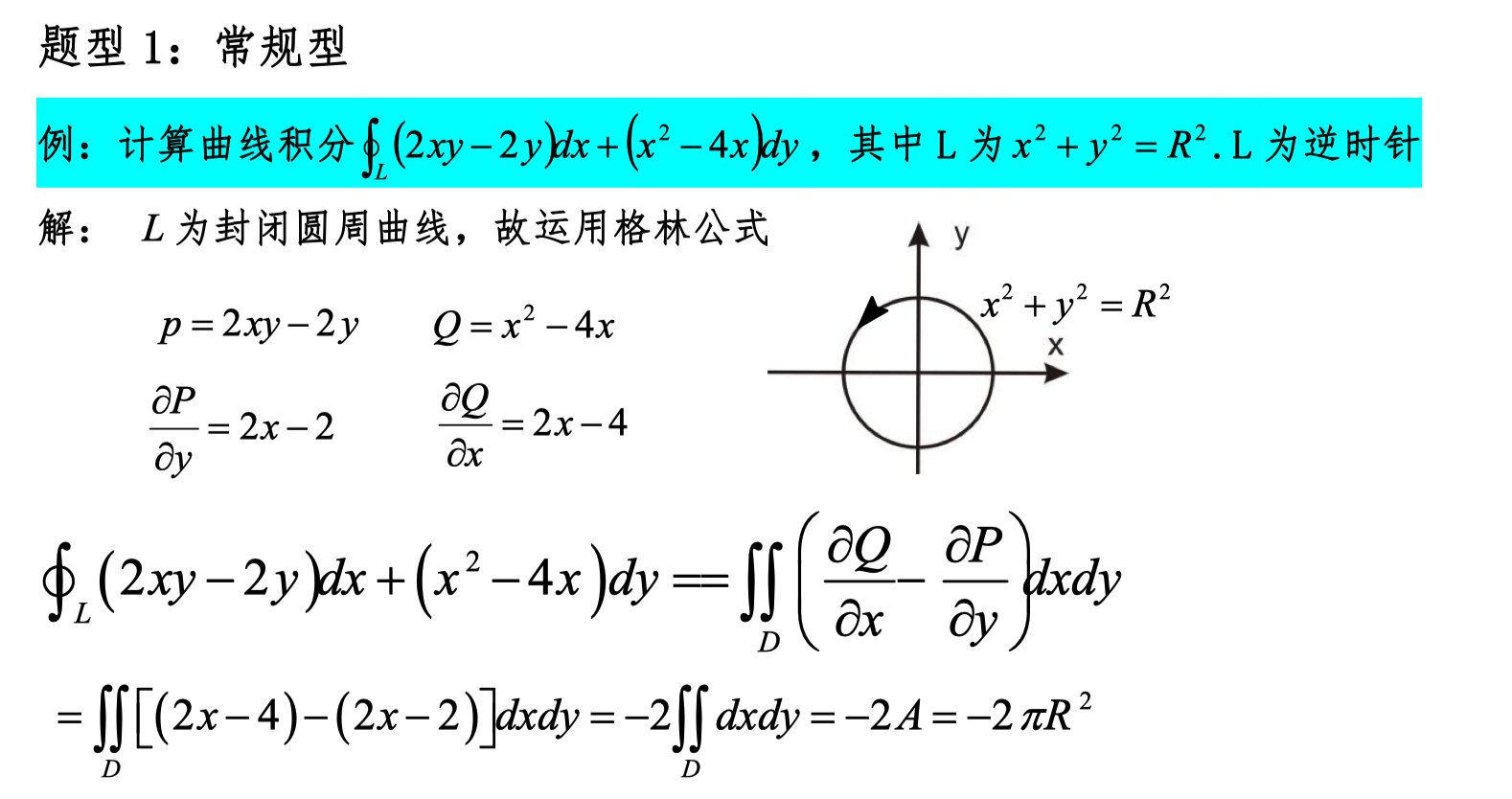
Most commonly tested problem type

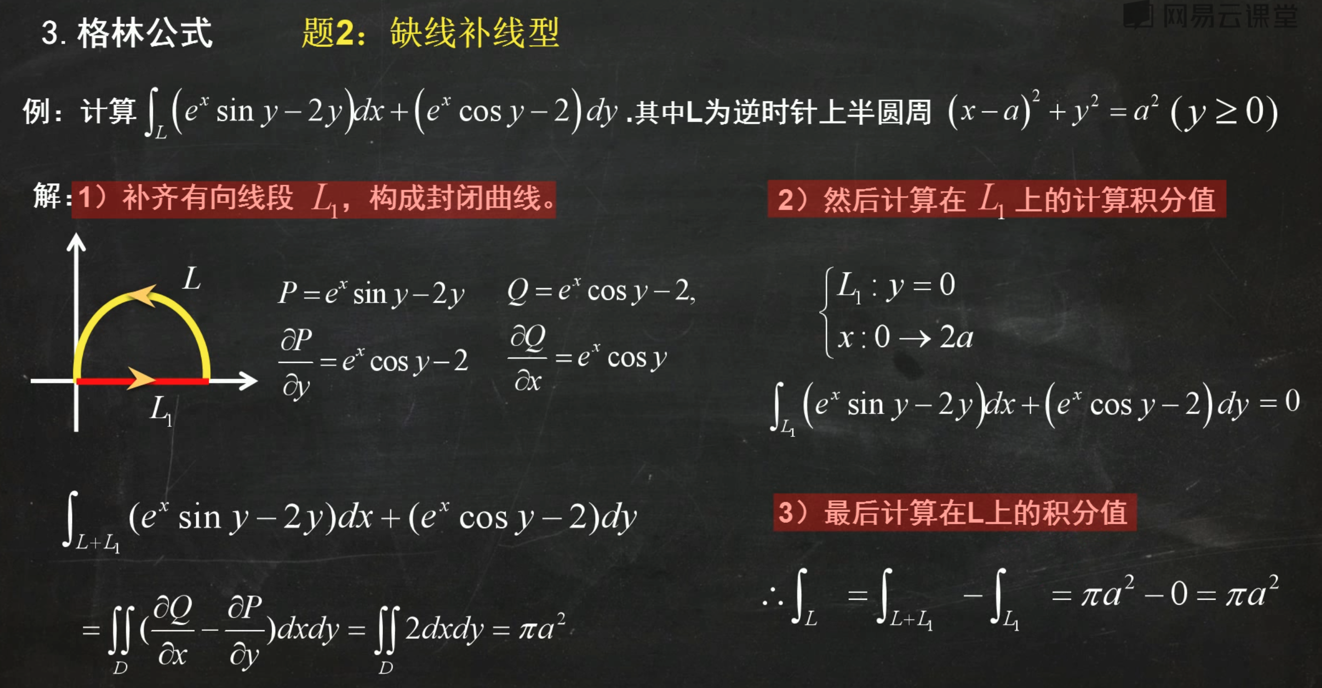
The integral region here does not have to be closed; you can also use the property that the integral is path-independent.

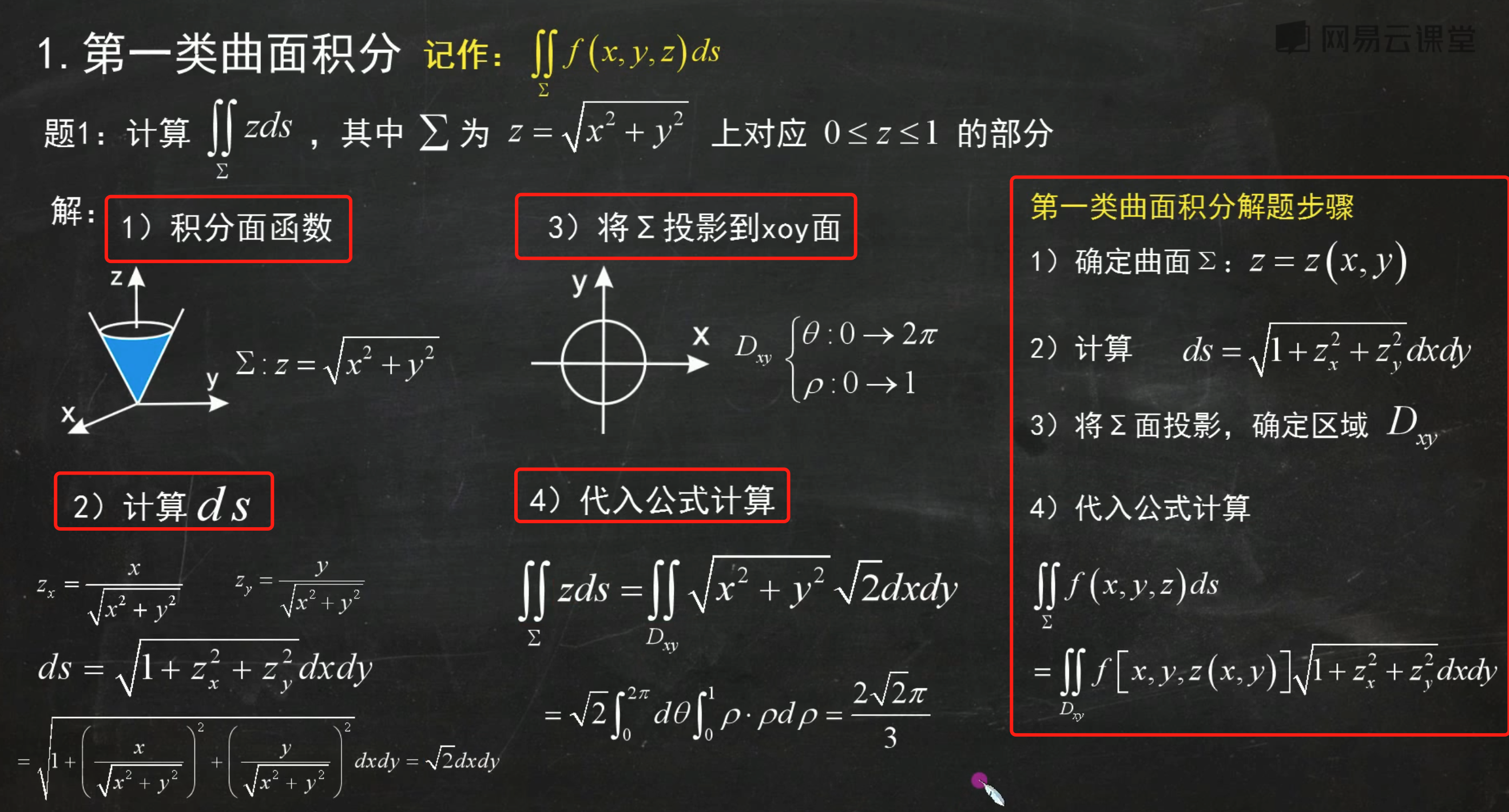
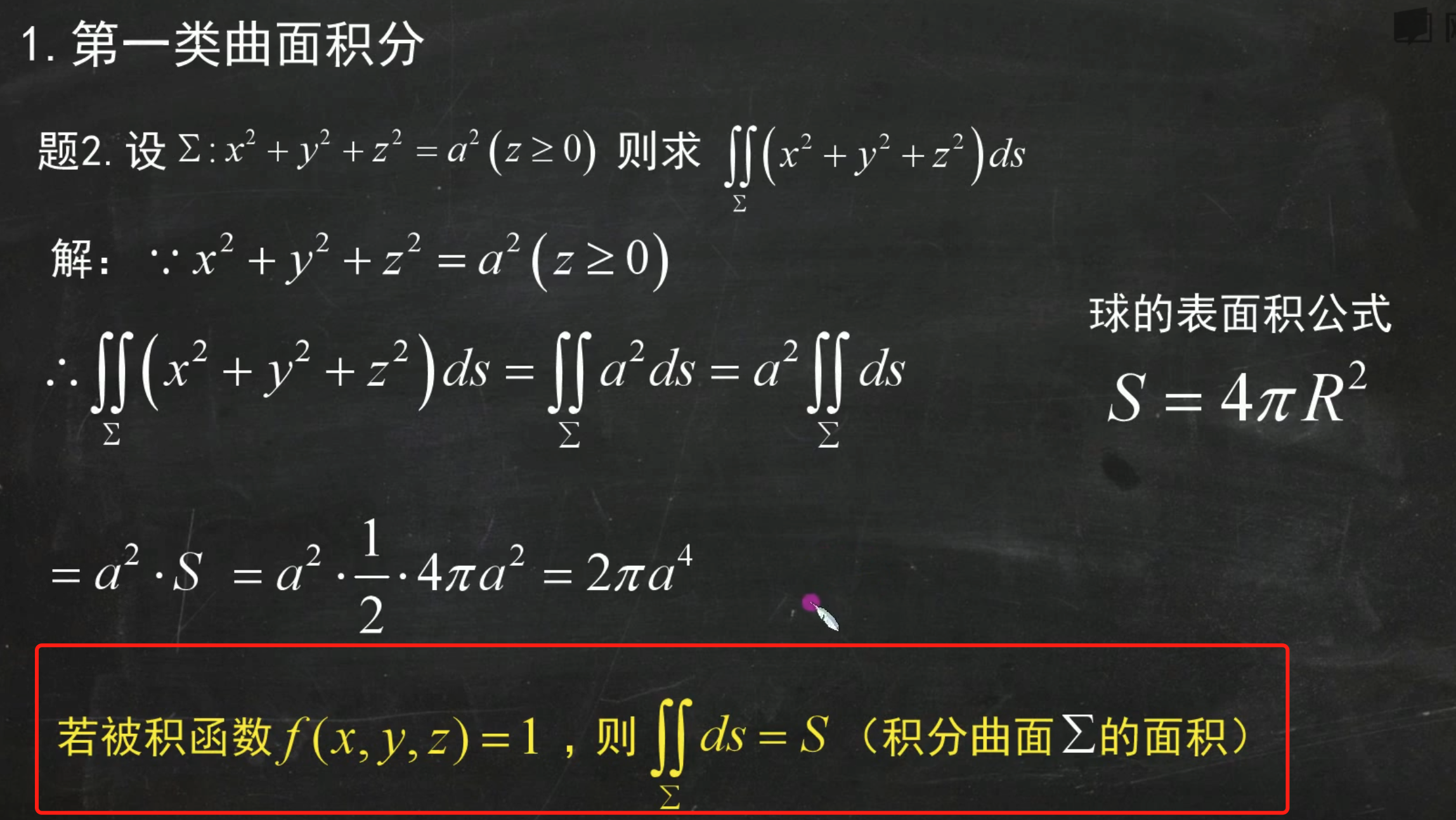
Surface Integrals of the First Kind

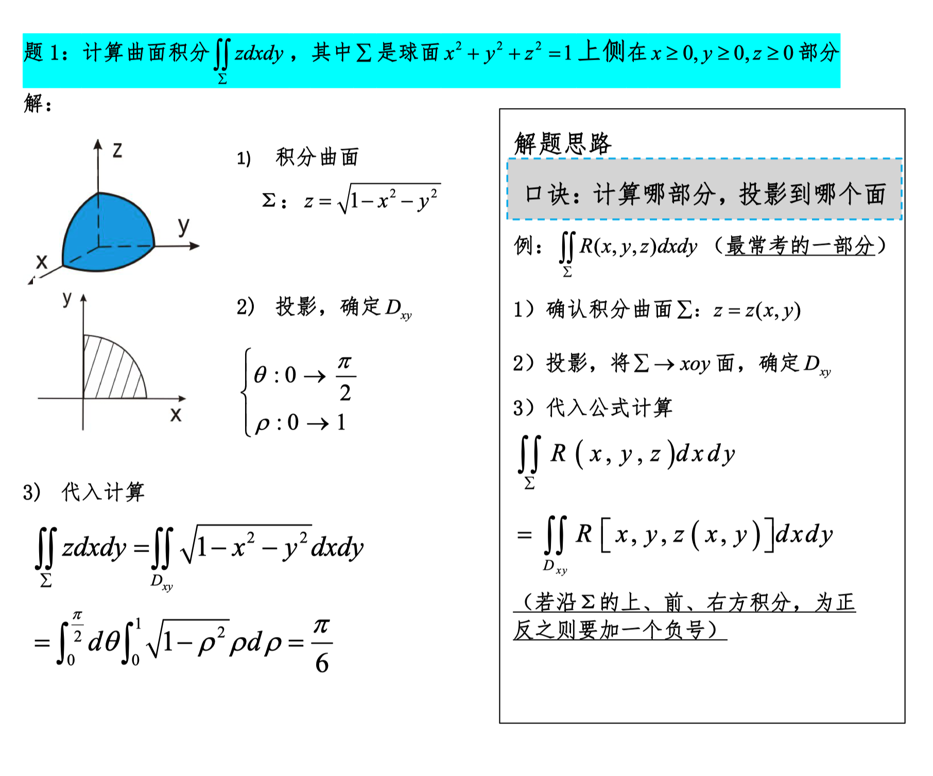
Surface Integrals of the Second Kind

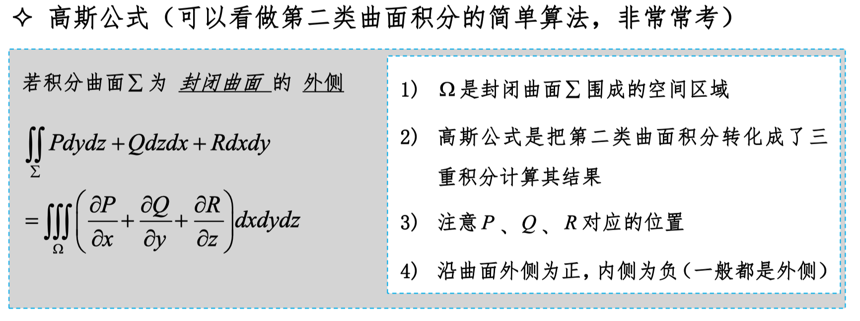
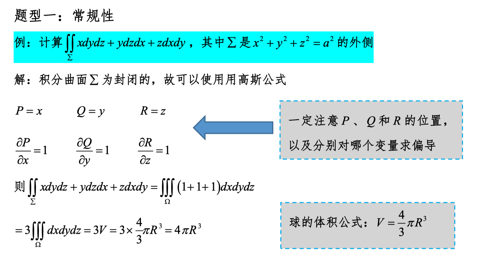
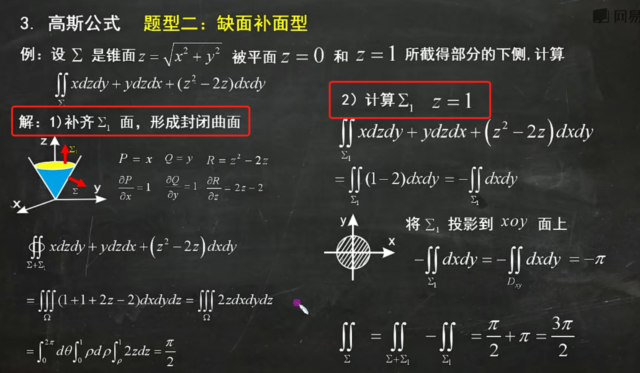
Gauss's Divergence Theorem

Series with Constant Terms

Series

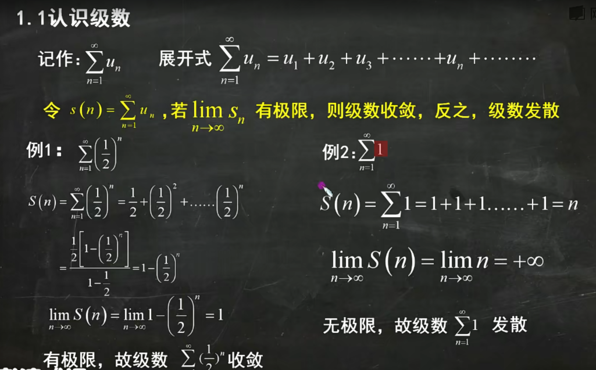
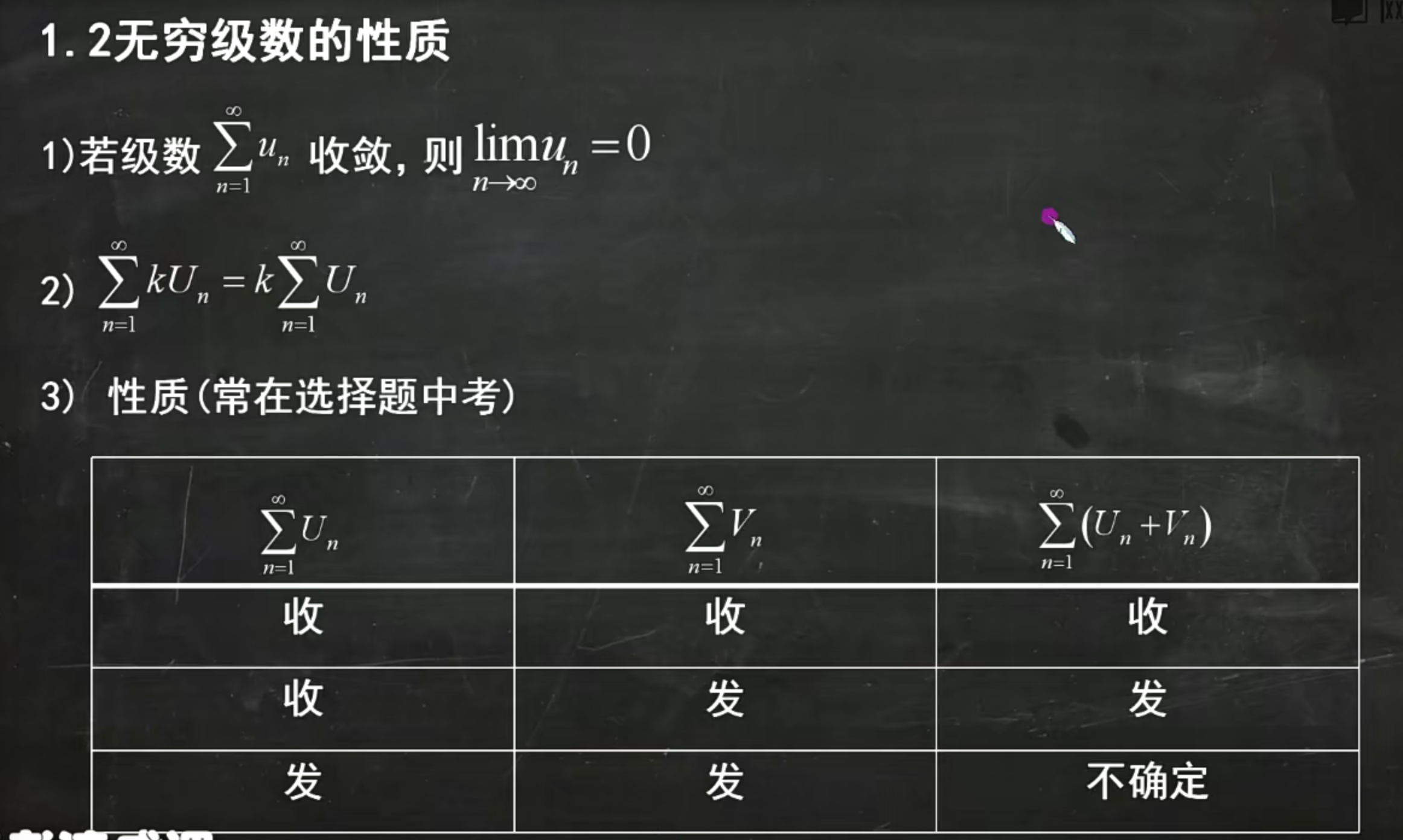
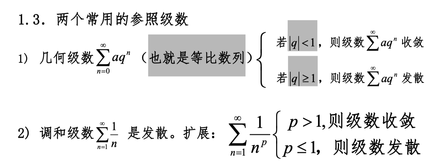
Convergence Tests

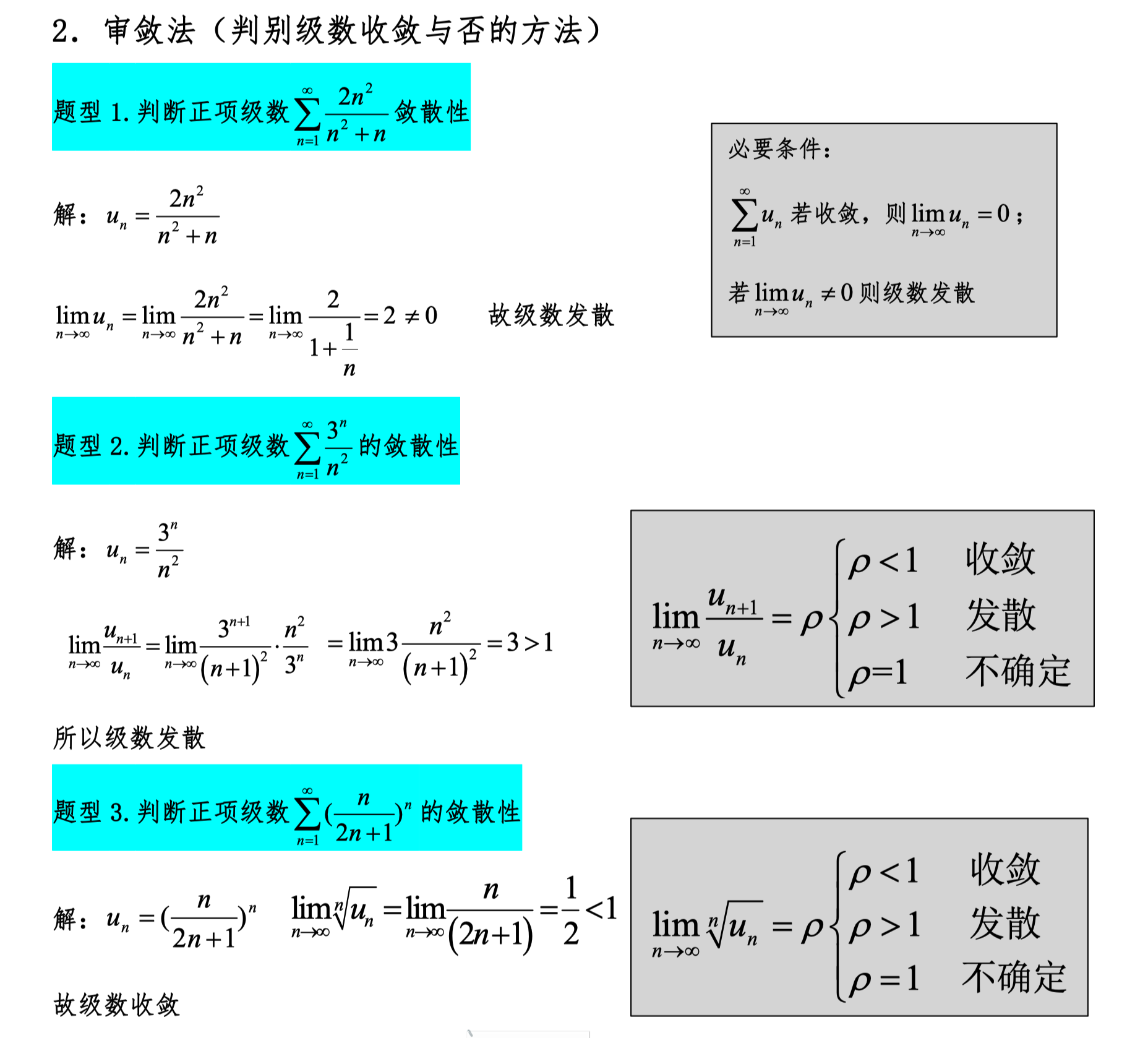
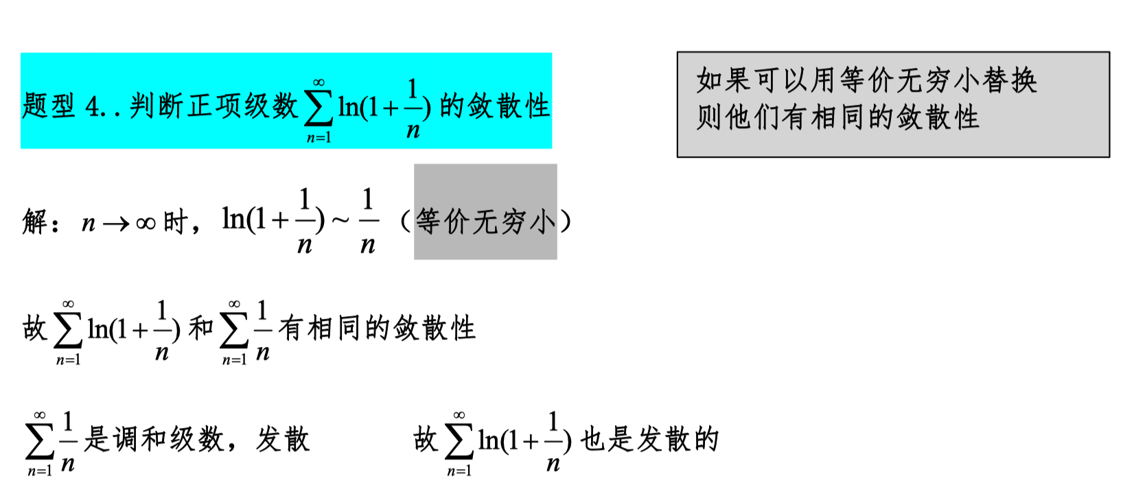
1. Use the necessary condition: as n approaches infinity, the general term equals 0.
2. Ratio test
3. Root test
4. Equivalent infinitesimal substitution

Alternating Series

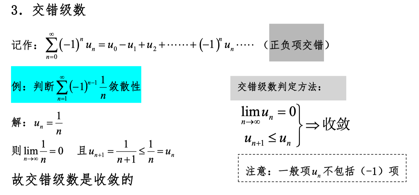
Two conditions for convergence:

1. As n approaches infinity, the general term approaches 0 (excluding the (-1) part).
2. Monotonically decreasing.

Absolute Convergence, Conditional Convergence

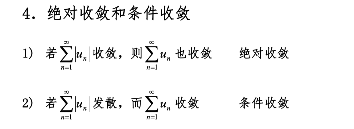
Both absolute convergence and conditional convergence mean the original expression converges; the difference is in the convergence behavior after taking the absolute value.

Power Series

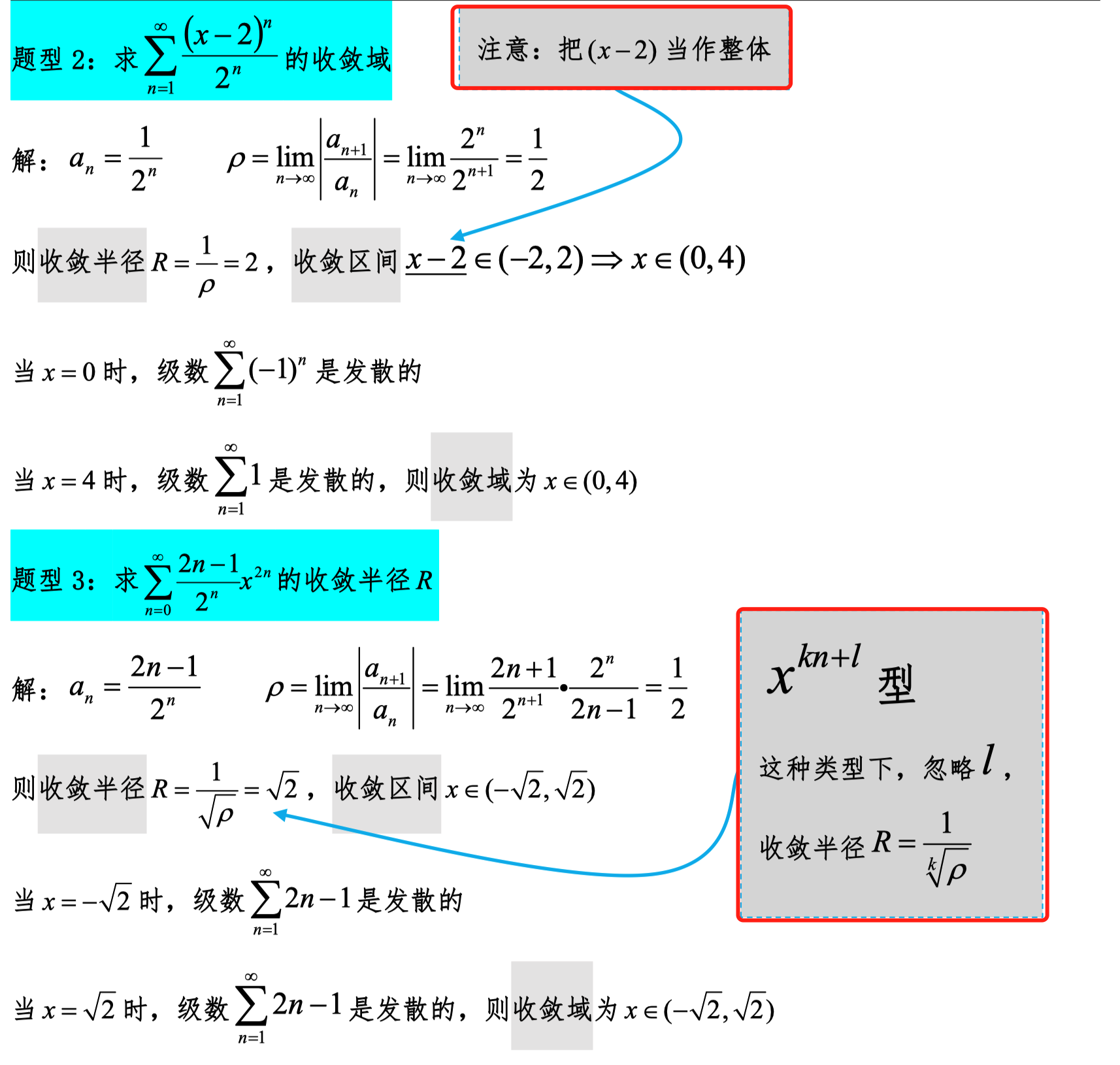
A series containing x terms is called a power series. The convergence and divergence of a power series depend on the value of x.

Radius of Convergence, Interval of Convergence

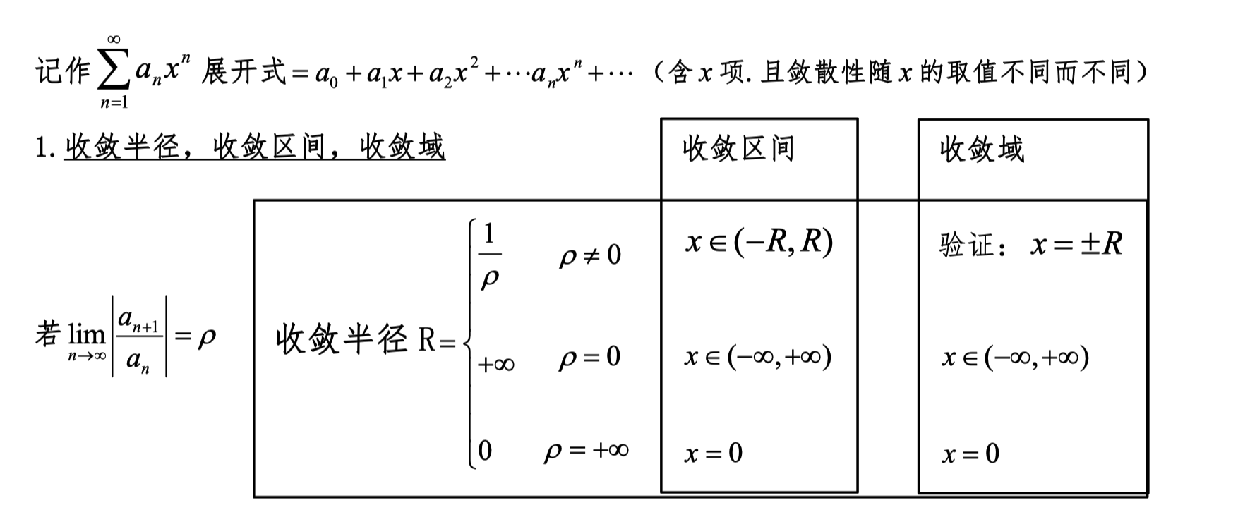
Note: The general term aₙ here refers to terms without x.

Both the convergence interval and the radius of convergence refer to the values of x.

When p ≠ 0, the boundaries of the convergence interval for x need to be substituted into the original expression for verification.

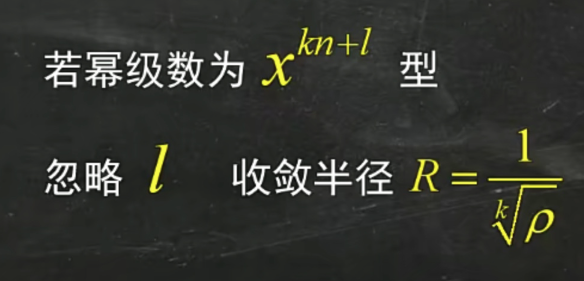
The formula in the image discusses the radius of convergence of a certain series. According to the content, the series term is of the form x^(kn+l), and the radius of convergence R is expressed as R = 1/ρ^(1/k).

The reason l can be ignored is: when discussing the convergence of a series, the l in the exponent has no substantial effect on the radius of convergence. In fact, the main factor affecting the series term is kn, because k and n determine the growth rate of the exponent, while l is a fixed offset that does not affect the overall convergence of the series.

In short, the convergence of the series mainly depends on kn, and ignoring l is because it does not change the convergence properties of the series or the calculation of the radius of convergence.

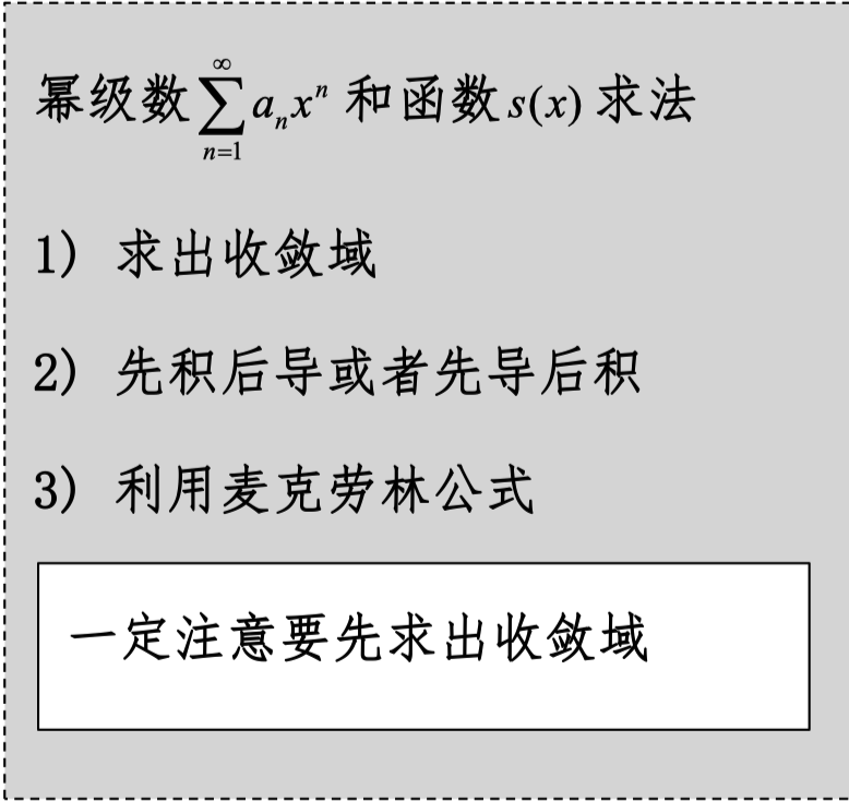
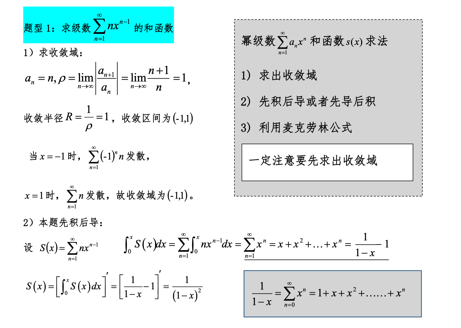
Sum Function

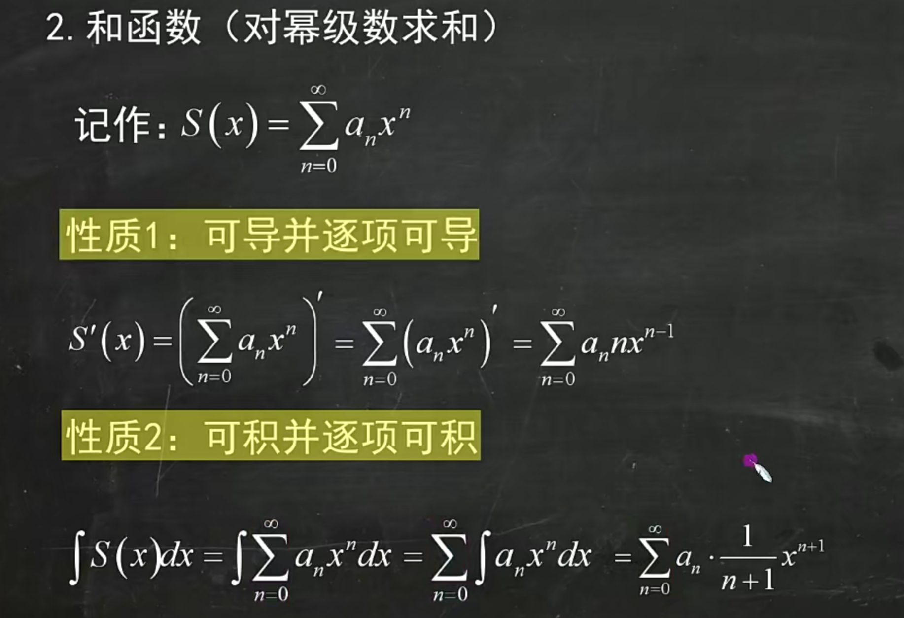
Note

When differentiating first and then integrating, or integrating first and then differentiating, don't forget the integration limits.

The upper limit is x and the lower limit is 0.

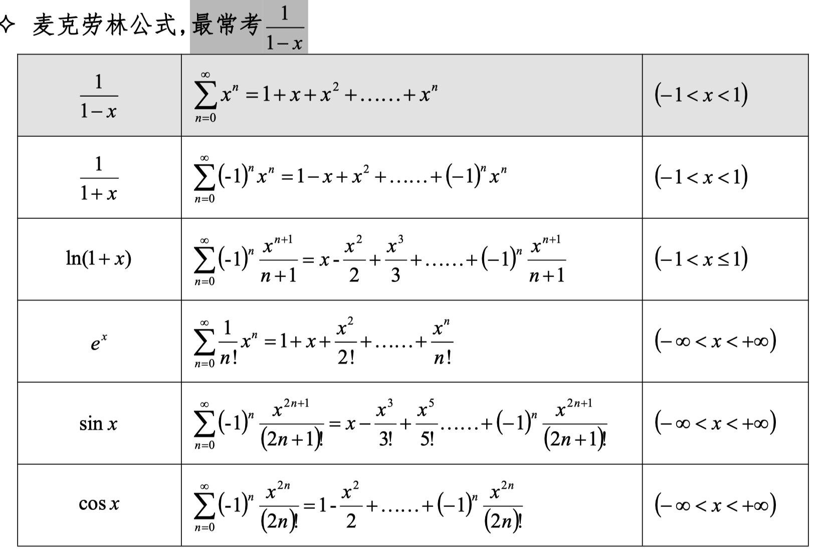
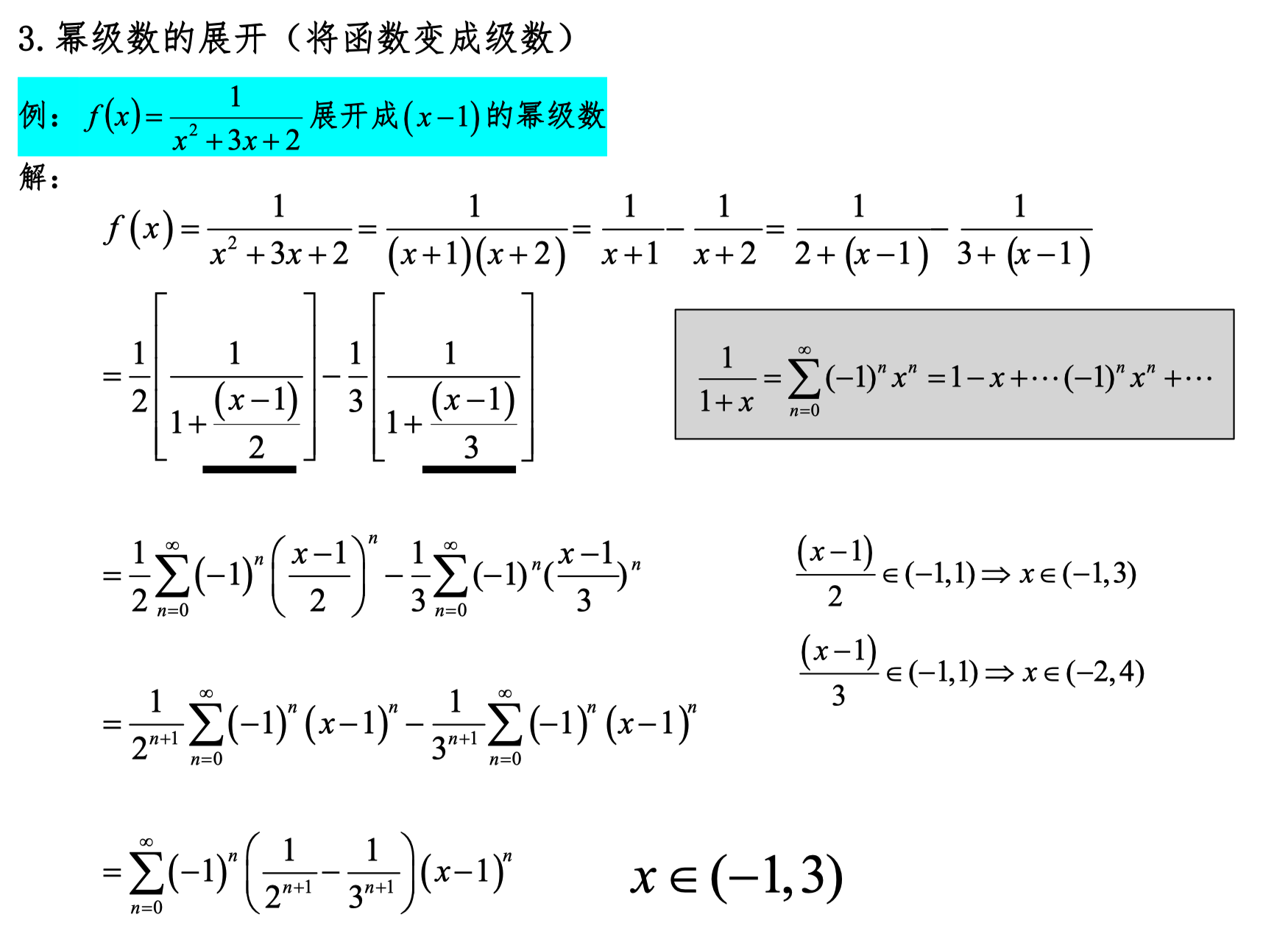
Power Series Expansion

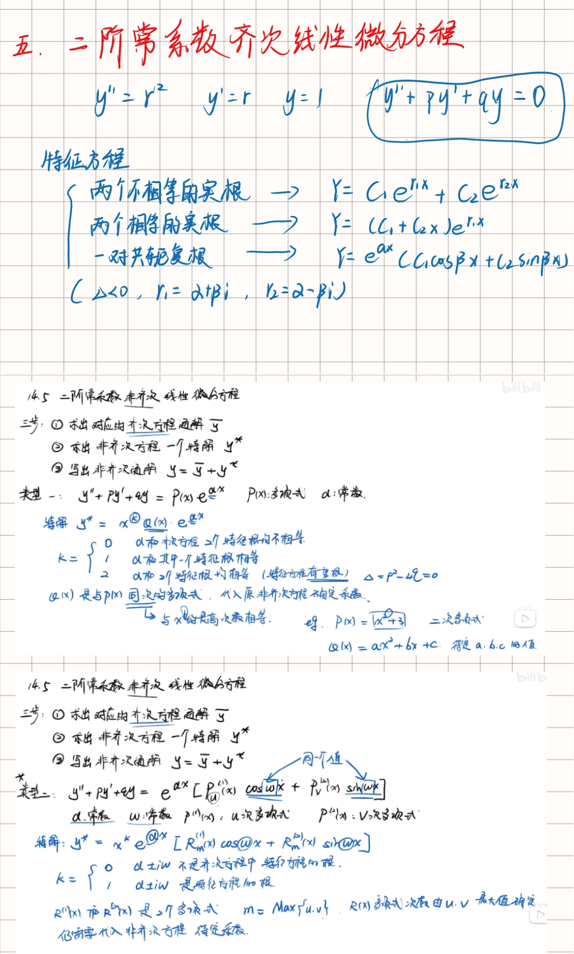
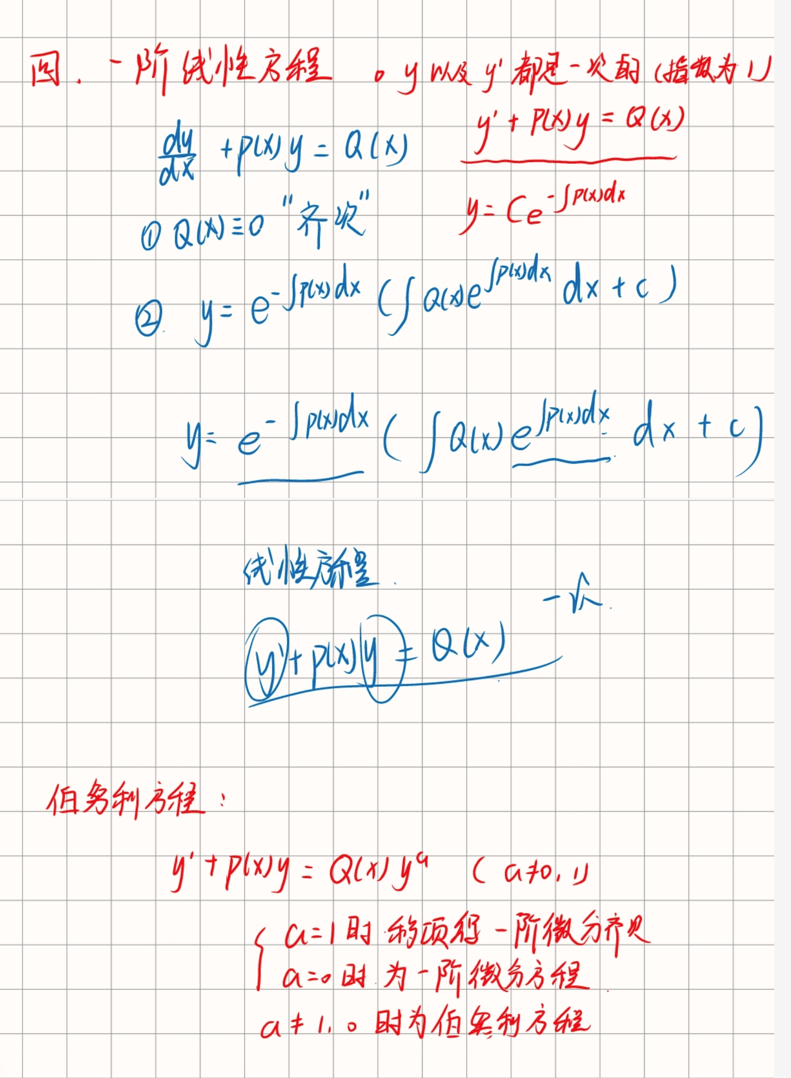
Differential Equations

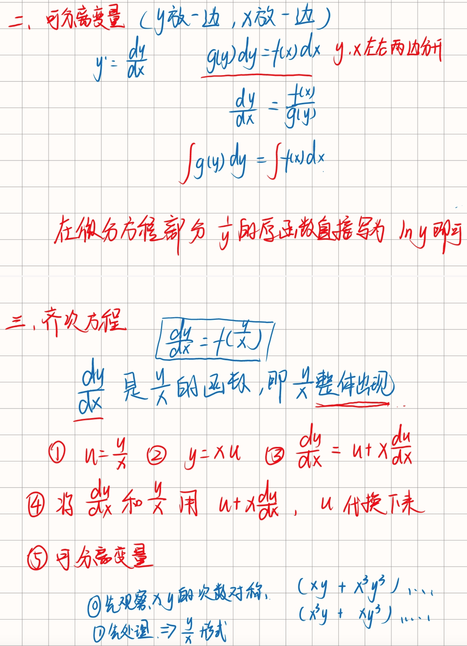
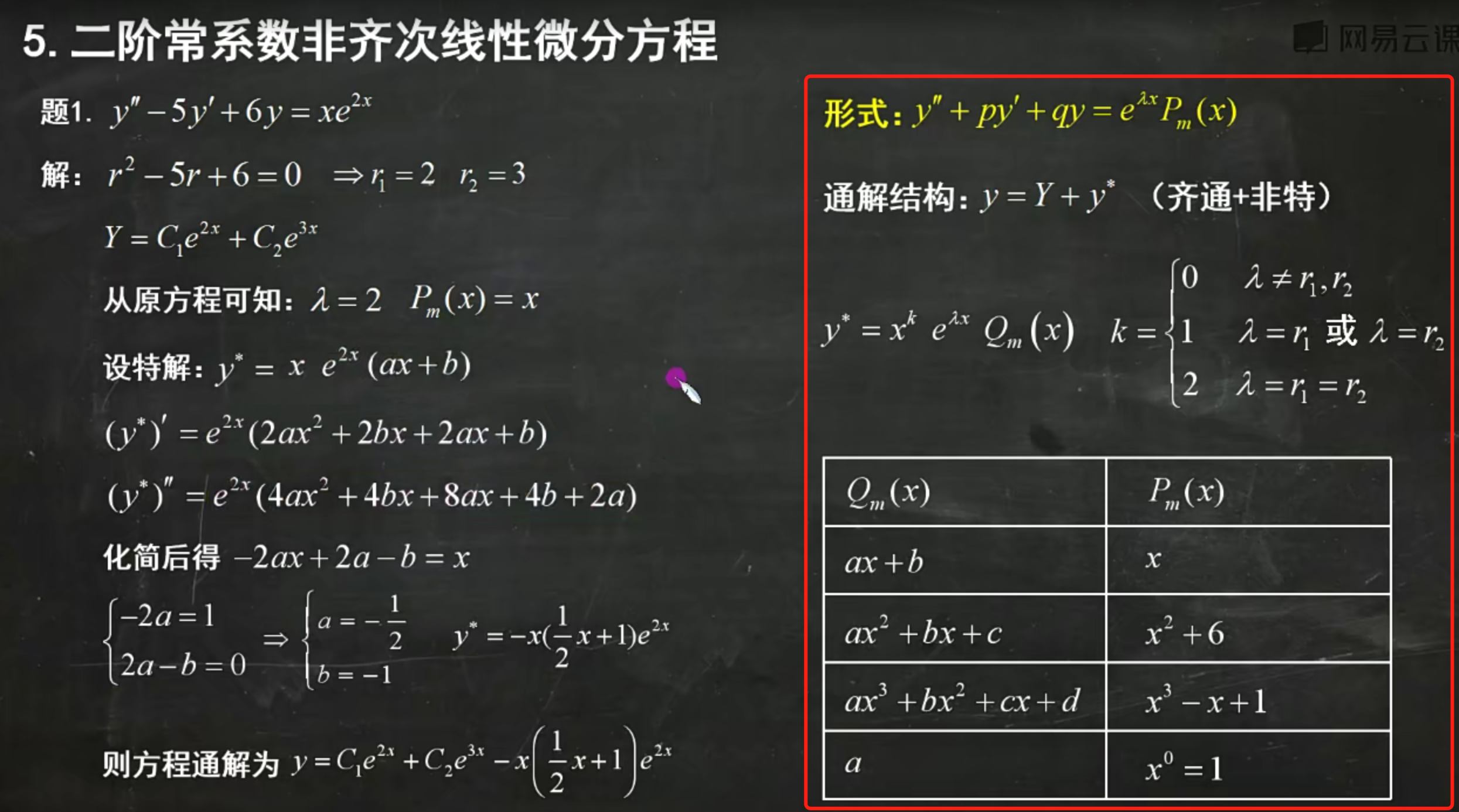
Find the homogeneous general solution.

Find the particular solution.

Differentiate the particular solution and substitute back to find unknowns (match corresponding terms).

Finally, add the homogeneous general solution and the particular solution to get the final answer.

Fourier Series

Linear Superposition Principle for Second-Order Linear Homogeneous Equations

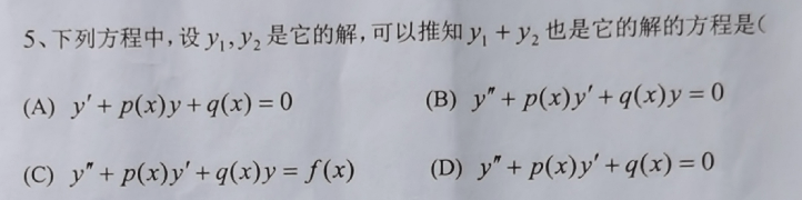
Second-order linear homogeneous differential equations have the property of linear superposition. To understand this in more detail, consider a general second-order linear homogeneous differential equation:

$$a(x) y'' + b(x) y' + c(x) y = 0$$

where a(x), b(x), and c(x) are functions of x, and y is the function to be solved.

Linear Superposition Principle

The linear superposition principle states that if y₁(x) and y₂(x) are two solutions of this second-order linear homogeneous differential equation, then their linear combination is also a solution. Specifically, for any constants C₁ and C₂, the function

$$y(x) = C_1 y_1(x) + C_2 y_2(x)$$

is also a solution of the original equation. We can verify this:

1. Compute the derivatives of y:

$$y' = C_1 y_1' + C_2 y_2'$$ $$y'' = C_1 y_1'' + C_2 y_2''$$

2. Substitute y, y', and y'' into the original equation:

$$a(x) y'' + b(x) y' + c(x) y = a(x) (C_1 y_1'' + C_2 y_2'') + b(x) (C_1 y_1' + C_2 y_2') + c(x) (C_1 y_1 + C_2 y_2)$$

3. Expand and rearrange:

$$= C_1 [a(x) y_1'' + b(x) y_1' + c(x) y_1] + C_2 [a(x) y_2'' + b(x) y_2' + c(x) y_2]$$

4. Since y₁ and y₂ are both solutions of the original equation:

$$a(x) y_1'' + b(x) y_1' + c(x) y_1 = 0$$ $$a(x) y_2'' + b(x) y_2' + c(x) y_2 = 0$$

5. Therefore:

$$C_1 \cdot 0 + C_2 \cdot 0 = 0$$

This shows that y = C₁y₁ + C₂y₂ is indeed a solution of the original equation.

Summary

Second-order linear homogeneous differential equations indeed have the property of linear superposition. This is an important property of linear differential equations that allows constructing new solutions from known solutions, greatly simplifying the problem-solving process.

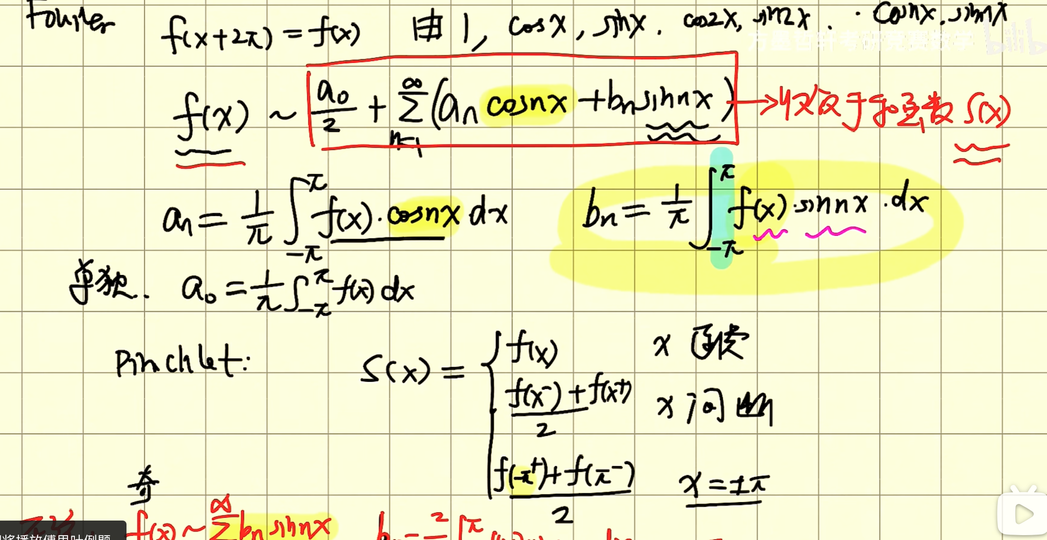
Introduction to Fourier Series

A Fourier series can represent a periodic function as a sum of sine and cosine functions. The Fourier series of a periodic function f(x) with period T is expressed as:

$$f(x) = a_0 + \sum_{n=1}^{\infty} \left( a_n \cos \left( \frac{2n\pi x}{T} \right) + b_n \sin \left( \frac{2n\pi x}{T} \right) \right)$$

where the formulas for a₀, aₙ, and bₙ are:

$$a_0 = \frac{1}{T} \int_{-T/2}^{T/2} f(x) \, dx$$ $$a_n = \frac{2}{T} \int_{-T/2}^{T/2} f(x) \cos \left( \frac{2n\pi x}{T} \right) \, dx$$ $$b_n = \frac{2}{T} \int_{-T/2}^{T/2} f(x) \sin \left( \frac{2n\pi x}{T} \right) \, dx$$

In this problem, T = 2, so the formulas become:

$$a_0 = \frac{1}{2} \int_{-1}^{1} f(x) \, dx$$ $$a_n = \int_{-1}^{1} f(x) \cos(n\pi x) \, dx$$ $$b_n = \int_{-1}^{1} f(x) \sin(n\pi x) \, dx$$

Finding a₀

$$a_0 = \frac{1}{2} \left( \int_{-1}^{0} 4 \, dx + \int_{0}^{1} x^2 \, dx \right)$$

Computing the integrals:

$$\int_{-1}^{0} 4 \, dx = 4x \Big|_{-1}^{0} = 4(0 - (-1)) = 4$$ $$\int_{0}^{1} x^2 \, dx = \frac{x^3}{3} \Big|_{0}^{1} = \frac{1}{3} - 0 = \frac{1}{3}$$

So:

$$a_0 = \frac{1}{2} \left( 4 + \frac{1}{3} \right) = \frac{1}{2} \cdot \frac{13}{3} = \frac{13}{6}$$

Finding aₙ

$$a_n = \int_{-1}^{0} 4 \cos(n\pi x) \, dx + \int_{0}^{1} x^2 \cos(n\pi x) \, dx$$

Computing these two integrals separately:

$$\int_{-1}^{0} 4 \cos(n\pi x) \, dx = \frac{4}{n\pi} \sin(n\pi x) \Big|_{-1}^{0} = \frac{4}{n\pi} (0 - (-\sin(n\pi))) = \frac{4\sin(n\pi)}{n\pi} = 0$$

because sin(nπ) = 0.

Next is the second integral:

$$\int_{0}^{1} x^2 \cos(n\pi x) \, dx$$

This integral requires integration by parts. We use integration by parts twice to solve it.

$$u = x^2, \quad dv = \cos(n\pi x) \, dx$$ $$du = 2x \, dx, \quad v = \frac{\sin(n\pi x)}{n\pi}$$

First integration:

$$\int x^2 \cos(n\pi x) \, dx = x^2 \cdot \frac{\sin(n\pi x)}{n\pi} \Big|_{0}^{1} - \int 2x \cdot \frac{\sin(n\pi x)}{n\pi} \, dx$$ $$= \frac{\sin(n\pi)}{n\pi} - 0 - \frac{2}{n\pi} \int x \sin(n\pi x) \, dx = 0 - \frac{2}{n\pi} \int x \sin(n\pi x) \, dx$$

Next, use integration by parts again:

$$u = x, \quad dv = \sin(n\pi x) \, dx$$ $$du = dx, \quad v = -\frac{\cos(n\pi x)}{n\pi}$$ $$\int x \sin(n\pi x) \, dx = -\frac{x \cos(n\pi x)}{n\pi} \Big|_{0}^{1} + \int \frac{\cos(n\pi x)}{n\pi} \, dx = -\frac{\cos(n\pi)}{n\pi^2} + \int \frac{\cos(n\pi x)}{n\pi} \, dx$$ $$= -\frac{(-1)^n}{n\pi^2} + \frac{\sin(n\pi x)}{(n\pi)^2} \Big|_{0}^{1} = -\frac{(-1)^n}{n\pi^2} + 0 = -\frac{(-1)^n}{n\pi^2}$$

So:

$$a_n = 0 - \frac{2}{n\pi} \cdot -\frac{(-1)^n}{n\pi^2} = \frac{2(-1)^n}{n^2 \pi^3}$$

Finding bₙ

Since f(x) is an even function, all bₙ are 0:

$$b_n = \int_{-1}^{1} f(x) \sin(n\pi x) \, dx = 0$$

Conclusion

$$f(x) = \frac{13}{6} + \sum_{n=1}^{\infty} \frac{2(-1)^n}{n^2 \pi^3} \cos(n\pi x)$$

Therefore, the Fourier series converges at x = 0 to:

$$f(0) = \frac{13}{6} + \sum_{n=1}^{\infty} \frac{2(-1)^n}{n^2 \pi^3} \cos(0) = \frac{13}{6} + \sum_{n=1}^{\infty} \frac{2(-1)^n}{n^2 \pi^3}$$

Since all bₙ = 0, the Fourier series result is the sum above.

Summary

Symmetry Properties of Various Integral Forms

Let's explore in detail the symmetry properties in different types of integrals and their effects.

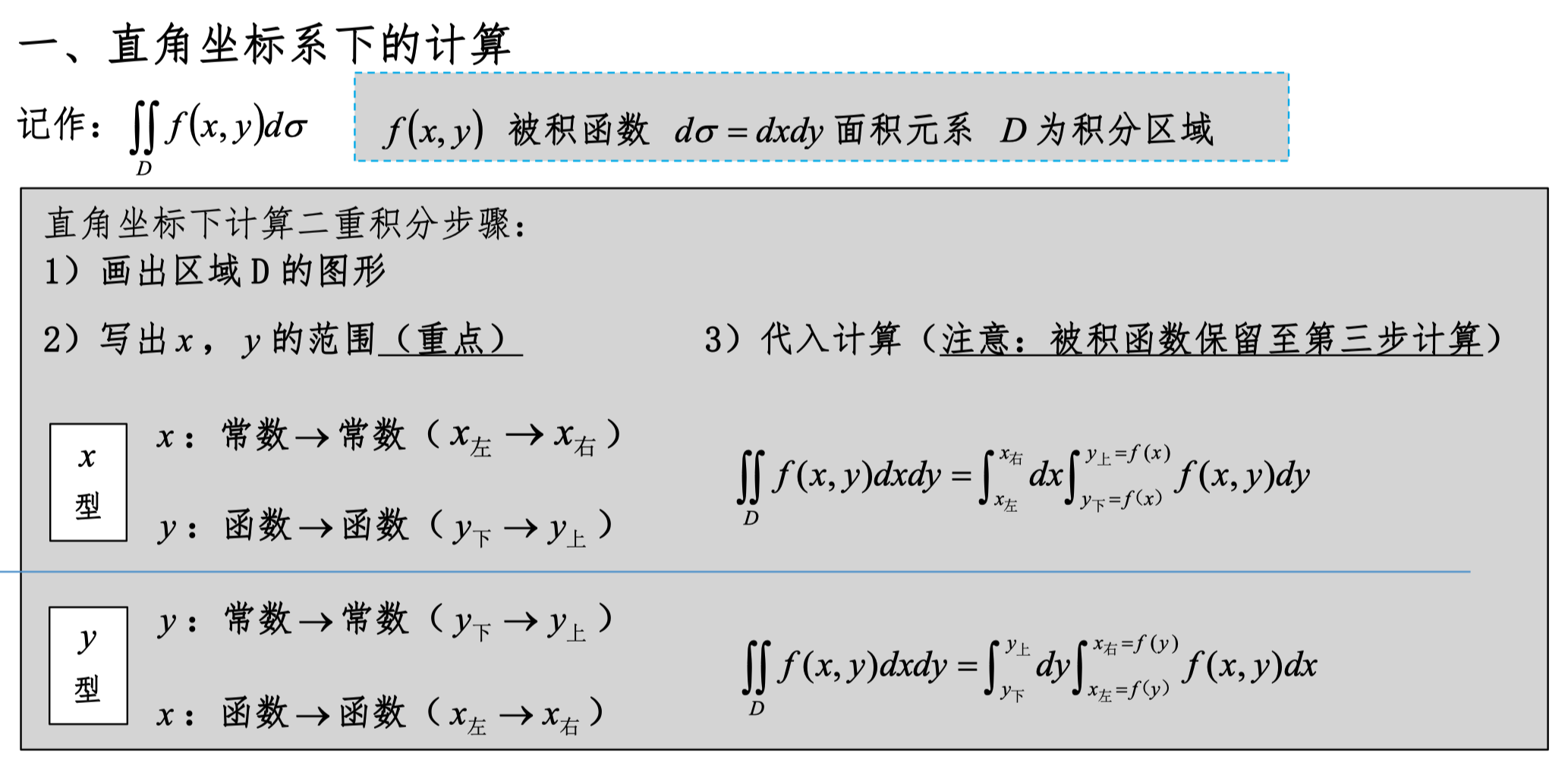
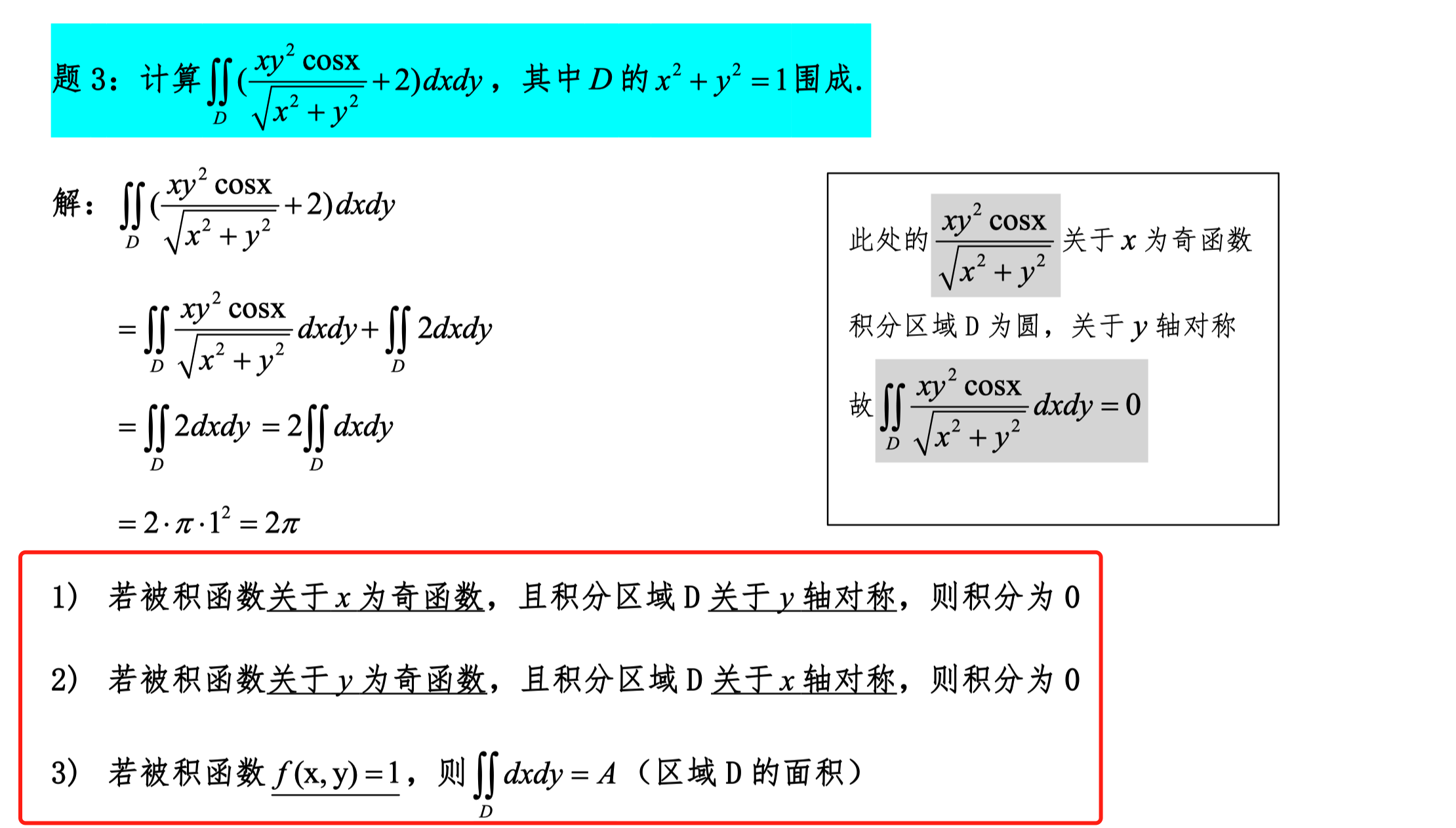
1. Double Integrals and Symmetry

For double integrals, if the integrand and integration region have specific symmetry, the integral result may be zero.

Definition of Double Integral:

$\iint_D f(x, y) \, dA$

Case 1: The integrand is an odd function with respect to x, and the integration region D is symmetric about the y-axis.

If $f(-x, y) = -f(x, y)$ and the integration region D is symmetric about the y-axis, then: $\iint_D f(x, y) \, dA = 0$ This is because on a symmetric region, the positive and negative parts of an odd function cancel each other out.

Case 2: The integrand is an odd function with respect to y, and the integration region D is symmetric about the x-axis.

If $f(x, -y) = -f(x, y)$ and the integration region D is symmetric about the x-axis, then: $\iint_D f(x, y) \, dA = 0$ The reason is the same — the positive and negative parts of an odd function cancel each other on a symmetric region.

2. Triple Integrals and Symmetry

Triple integrals have similar properties.

Definition of Triple Integral:

$\iiint_V f(x, y, z) \, dV$

Case 1: The integrand is an odd function with respect to x, and the integration region V is symmetric about the y-axis.

If $f(-x, y, z) = -f(x, y, z)$ and the integration region V is symmetric about the y-axis, then: $\iiint_V f(x, y, z) \, dV = 0$

Case 2: The integrand is an odd function with respect to y, and the integration region V is symmetric about the x-axis.

If $f(x, -y, z) = -f(x, y, z)$ and the integration region V is symmetric about the x-axis, then: $\iiint_V f(x, y, z) \, dV = 0$

3. Line Integrals of the First Kind and Symmetry

Line integrals of the first kind integrate a scalar field along a given path.

Definition:

$\int_C f(x, y) \, ds$

For line integrals of the first kind, if the integrand f and path C have specific symmetry, the integral may also be zero.

Case 1: The integrand is an odd function with respect to x, and path C is symmetric about the y-axis.

If $f(-x, y) = -f(x, y)$ and path C is symmetric about the y-axis, then: $\int_C f(x, y) \, ds = 0$

Case 2: The integrand is an odd function with respect to y, and path C is symmetric about the x-axis.

If $f(x, -y) = -f(x, y)$ and path C is symmetric about the x-axis, then: $\int_C f(x, y) \, ds = 0$

4. Line Integrals of the Second Kind and Symmetry

Line integrals of the second kind integrate a vector field along a given path.

Definition:

$\int_C \mathbf{F} \cdot d\mathbf{r}$

For line integrals of the second kind, the symmetry of the vector field $\mathbf{F}$ and the symmetry of path C can also lead to zero integral results.

Case 1: The vector field is an odd function with respect to x, and path C is symmetric about the y-axis.

If $\mathbf{F}(-x, y) = -\mathbf{F}(x, y)$ and path C is symmetric about the y-axis, then: $\int_C \mathbf{F} \cdot d\mathbf{r} = 0$

Case 2: The vector field is an odd function with respect to y, and path C is symmetric about the x-axis.

If $\mathbf{F}(x, -y) = -\mathbf{F}(x, y)$ and path C is symmetric about the x-axis, then: $\int_C \mathbf{F} \cdot d\mathbf{r} = 0$

5. Surface Integrals of the First Kind and Symmetry

Surface integrals of the first kind integrate a scalar field over a surface.

Definition:

$\iint_S f(x, y, z) \, dS$

For surface integrals of the first kind, if the integrand f and surface S have specific symmetry, the integral result may also be zero.

Case 1: The integrand is an odd function with respect to x, and surface S is symmetric about the y-axis.

If $f(-x, y, z) = -f(x, y, z)$ and surface S is symmetric about the y-axis, then: $\iint_S f(x, y, z) \, dS = 0$

Case 2: The integrand is an odd function with respect to y, and surface S is symmetric about the x-axis.

If $f(x, -y, z) = -f(x, y, z)$ and surface S is symmetric about the x-axis, then: $\iint_S f(x, y, z) \, dS = 0$

6. Surface Integrals of the Second Kind and Symmetry

Surface integrals of the second kind integrate a vector field over a surface.

Definition:

$\iint_S \mathbf{F} \cdot d\mathbf{S}$

For surface integrals of the second kind, if the vector field $\mathbf{F}$ and surface S have specific symmetry, the integral result may also be zero.

Case 1: The vector field is an odd function with respect to x, and surface S is symmetric about the y-axis.

If $\mathbf{F}(-x, y, z) = -\mathbf{F}(x, y, z)$ and surface S is symmetric about the y-axis, then: $\iint_S \mathbf{F} \cdot d\mathbf{S} = 0$

Case 2: The vector field is an odd function with respect to y, and surface S is symmetric about the x-axis.

If $\mathbf{F}(x, -y, z) = -\mathbf{F}(x, y, z)$ and surface S is symmetric about the x-axis, then: $\iint_S \mathbf{F} \cdot d\mathbf{S} = 0$

In summary, the property that integral results are zero under specific symmetry conditions is universal across all integral forms. The key lies in the odd-even nature of the integrand (or vector field) and the symmetry of the integration region (path or surface).

Derivative Formula for Integrals with Variable Limits

The derivative formula for integrals with variable limits involves the application of the Riemann-Stieltjes integral and the Fundamental Theorem of Calculus. Specifically, for an integral with variable limits:

$F(x) = \int_{a(x)}^{b(x)} f(t) \, dt$

The derivative formula is:

$$\frac{dF(x)}{dx} = f(b(x)) \cdot b'(x) - f(a(x)) \cdot a'(x) + \int_{a(x)}^{b(x)} \frac{\partial f(t, x)}{\partial x} \, dt$$

Here, a(x) and b(x) are the upper and lower limits of the integral, both functions of x, and f(t, x) is the integrand, which may also depend on x.

Specific steps:

1. Determine the derivatives of the limits: Compute the derivatives of a(x) and b(x) with respect to x, denoted a'(x) and b'(x).
2. Direct differentiation part of the integrand: If the integrand f(t, x) depends on x, compute its partial derivative with respect to x, ∂f(t,x)/∂x.
3. Apply the formula: Substitute all parts into the formula above.

For example, consider a specific case:

$F(x) = \int_{x}^{2x} \sin(t) \, dt$

1. Derivatives of limits:

   • a(x) = x, a'(x) = 1
   • b(x) = 2x, b'(x) = 2

2. Direct differentiation part of the integrand: sin(t) does not depend on x, so ∂sin(t)/∂x = 0.

3. Apply the formula:

$$\frac{dF(x)}{dx} = \sin(2x) \cdot 2 - \sin(x) \cdot 1 + \int_{x}^{2x} 0 \, dt = 2\sin(2x) - \sin(x)$$

So the derivative of F(x) is:

$$\frac{dF(x)}{dx} = 2\sin(2x) - \sin(x)$$

This gives us the derivative result for the integral with variable limits.

Computing Integrals of Functions $xe^x$, $xe^{-x}$, $-xe^x$, and $-xe^{-x}$

Using integration by parts

1. For $xe^x$:

   $$\int xe^x \, dx$$

   Using the integration by parts formula $\int u \, dv = uv - \int v \, du$, let $u = x$, $dv = e^x \, dx$, then $du = dx$, $v = e^x$. Thus:

   $$\int xe^x \, dx = xe^x - \int e^x \, dx = xe^x - e^x + C = e^x(x - 1) + C$$

2. For $xe^{-x}$:

   $$\int xe^{-x} \, dx$$

   Similarly, let $u = x$, $dv = e^{-x} \, dx$, then $du = dx$, $v = -e^{-x}$. Thus:

   $$\int xe^{-x} \, dx = -xe^{-x} - \int -e^{-x} \, dx = -xe^{-x} + e^{-x} + C = -e^{-x}(x + 1) + C$$

3. For $-xe^x$:

   $$\int -xe^x \, dx$$

   This is actually the negative of the integral of $xe^x$, so:

   $$\int -xe^x \, dx = -(e^x(x - 1)) + C = -e^x(x - 1) + C$$

4. For $-xe^{-x}$:

   $$\int -xe^{-x} \, dx$$

   This is actually the negative of the integral of $xe^{-x}$, so:

   $$\int -xe^{-x} \, dx = -(-e^{-x}(x + 1)) + C = e^{-x}(x + 1) + C$$

In summary, the integrals are:

1. $\int xe^x \, dx = e^x(x - 1) + C$
2. $\int xe^{-x} \, dx = -e^{-x}(x + 1) + C$
3. $\int -xe^x \, dx = -e^x(x - 1) + C$
4. $\int -xe^{-x} \, dx = e^{-x}(x + 1) + C$