Ding Zhiyu Winter Break Study Report

PPT

Decomposition Techniques and Decomposition Strategies

Decomposition techniques and decomposition strategies are two related but distinct concepts in parallel computing. Decomposition techniques involve dividing a problem into parts that can be processed in parallel, while decomposition strategies refer to how these parts are assigned to different processors or computing resources. Below is a detailed explanation of both:

Decomposition Techniques

Decomposition techniques are a core concept in parallel computing. They determine how to split a large problem into smaller problems for parallel processing. There are three main decomposition techniques:

1. Domain Decomposition: This technique divides the entire computational domain (such as a physical space, time interval, or data set) into several subdomains. Each subdomain can be individually assigned to a processor for computation. For example, when simulating a weather system, different regions of the atmospheric model can be assigned to different processors.

2. Functional Decomposition: In this technique, different functions or tasks are assigned to different processors. Each processor executes a specific function or task, which may be parallel or sequential. For example, in a video processing pipeline, one processor may handle decoding, another may handle rendering, and yet another may handle compression.

3. Data Decomposition: This technique involves dividing a data set into smaller parts that can be independently processed in parallel. For example, when processing a large array, the array can be divided into multiple blocks, each processed by a different processor.

Decomposition Strategies

Decomposition strategies determine how decomposed tasks or data blocks are assigned to processors. This strategy is crucial for load balancing, reducing communication overhead, and improving parallel efficiency. The main decomposition strategies include:

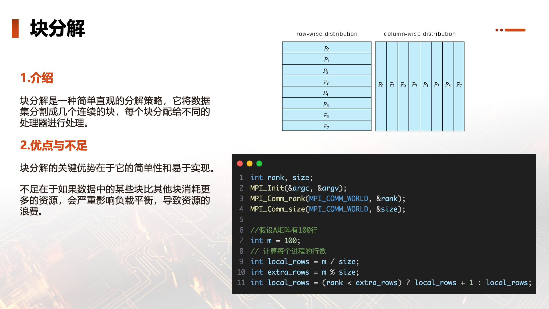
1. Block Decomposition: Divides the data set or task into equal-sized blocks, with each processor handling one or more blocks. This strategy is simple and easy to implement but may not be flexible enough for dynamically changing loads.

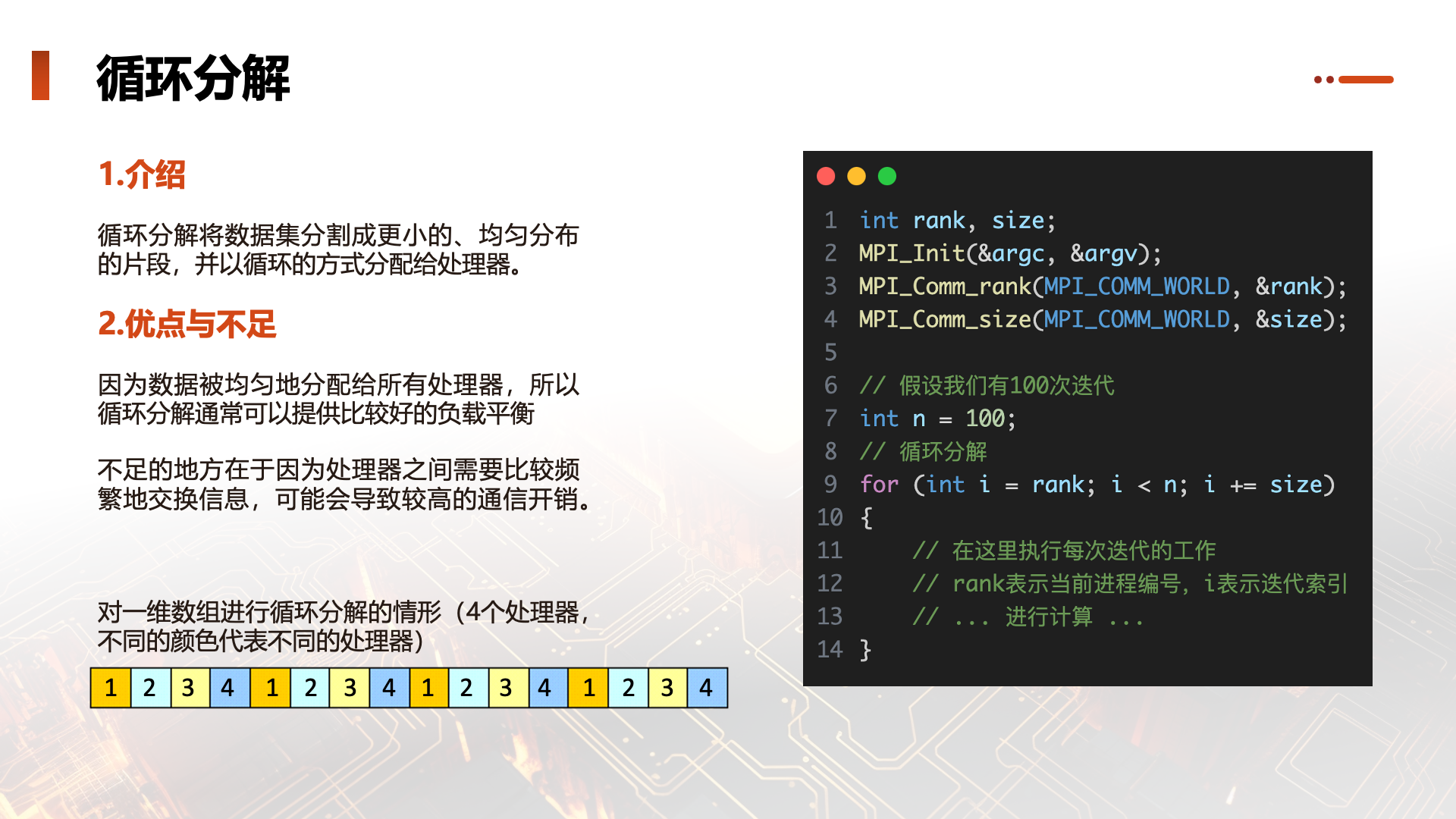
2. Cyclic Decomposition: The data set is divided into smaller blocks and assigned to processors in a round-robin fashion. This method can provide better load balancing, especially when processing time is difficult to predict.

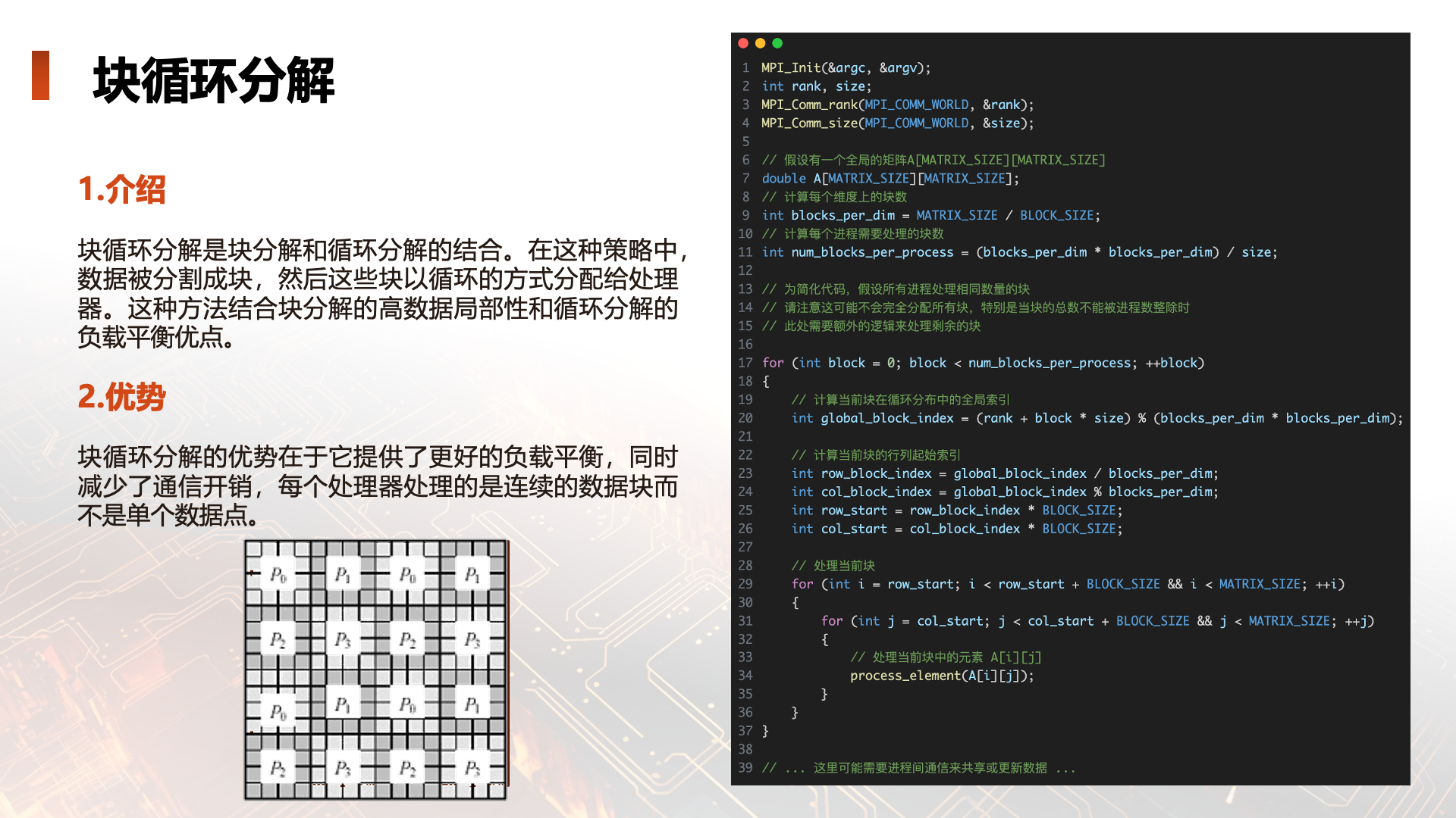
3. Block-Cyclic Decomposition: Combines the characteristics of block decomposition and cyclic decomposition. The data set is divided into equal-sized blocks, and then these blocks are assigned to processors in a round-robin fashion. This strategy attempts to balance load and reduce communication overhead.

In practice, choosing the appropriate decomposition technique and strategy depends on the nature of the problem, the characteristics of the computing resources, and the performance optimization goals. For example, if communication costs between processors are high, a decomposition strategy that reduces communication requirements may be preferred. If task execution times vary greatly, a more flexible load balancing strategy is needed.

When designing parallel programs, it is usually necessary to consider both decomposition techniques and decomposition strategies to ensure program efficiency and scalability. In fact, these two influence each other: choosing a certain decomposition technique may limit the available decomposition strategies, and vice versa. Therefore, developers need a deep understanding of both the problem and the computing environment to choose the most appropriate approach.

Decomposition Techniques

Introduction

A fundamental step in designing parallel algorithms is describing the computations needed to complete a given task and decomposing these computations into a set of subtasks that can be executed in parallel. For many problems, their task graphs contain sufficient parallelism. For such task graphs, tasks can be scheduled across multiple processors, allowing the problem to be completed in parallel. Unfortunately, many problems' task graphs do not exhibit such rich (or intuitive) parallelism. Instead, they often contain one task or multiple tasks that need to be executed serially. For such problems, we need to decompose the total computation task into a set of subtasks that can be executed in parallel. This process is called task decomposition. A good task decomposition should have the following characteristics:

　　☆ It should have a high degree of parallelism. Higher parallelism means the decomposed tasks can be executed in parallel on more processors. 　　☆ Interaction (communication and synchronization) between subtasks should be minimized. Less interaction means processors can focus more on the task itself rather than on additional computation and waiting caused by communication and synchronization.

　　In many cases, these two requirements conflict, meaning that task decomposition with high parallelism usually requires extensive interaction between subtasks. How to balance this conflict is an art in parallel algorithm design. This section mainly considers how to improve subtask parallelism, while discussion of interaction between subtasks is in the next section.

　　Below are several commonly used methods for task decomposition. For different problems, these methods are not always feasible and may not always yield the most optimal parallel algorithm. However, for many problems, these methods can provide a good "starting point" for parallelization.

　　Among these, recursive decomposition and data decomposition can be considered relatively general decomposition methods because they can be used for task decomposition of most problems, while search decomposition is more specialized and can only be applied to certain types of problems.

Recursive Decomposition Technique

Recursive decomposition is typically used for task decomposition of problems that use the Divide-and-conquer approach. This method decomposes tasks into independent subtasks, and the decomposition process recurses. The answer to the problem is the combination of all subtask answers. The divide-and-conquer strategy exhibits a natural parallelism.

Example: Quicksort

Quicksort a sequence A of n elements. Quicksort is a divide-and-conquer algorithm. The algorithm first selects a pivot element x, then divides A into two subsequences A0 and A1, where all elements in A0 are less than x, and all elements in A1 are greater than or equal to x. This is the partitioning part of the algorithm. The obtained subsequences are recursively subjected to the above partitioning process, and then the sorted subsequences are combined into the final result sequence A'. The quicksort process can be illustrated by the following diagram.

　　The dark-colored elements are the selected pivot elements. 　　Now consider how to perform task decomposition on the quicksort algorithm based on its divide-and-conquer characteristics. As can be seen from the diagram above, at each level of the task tree, the continued splitting of each subtask can be performed in parallel, and they are independent of each other. Therefore, the decomposition of the computation is actually also a tree. At the start of the algorithm, there is only one sequence (the root node of the tree), and we use one processor to perform its first partitioning. After partitioning, we get 2 subsequences at the first level. The partitioning of these two subsequences can be performed on two processors respectively. (If the sequences are long enough) at level i of the tree, there will be 2i subsequences, which can be independently and parallel completed by 2i processors.

Data Decomposition Technique

For algorithms with large data structures, data decomposition is a very useful method. It can be divided into two steps. In the first step, the data (or domain) on which computation operates is partitioned. In the second step, the corresponding computations are organized into subtasks based on the data partition. Data partitioning can be performed using the following methods.

Partitioning Output Data

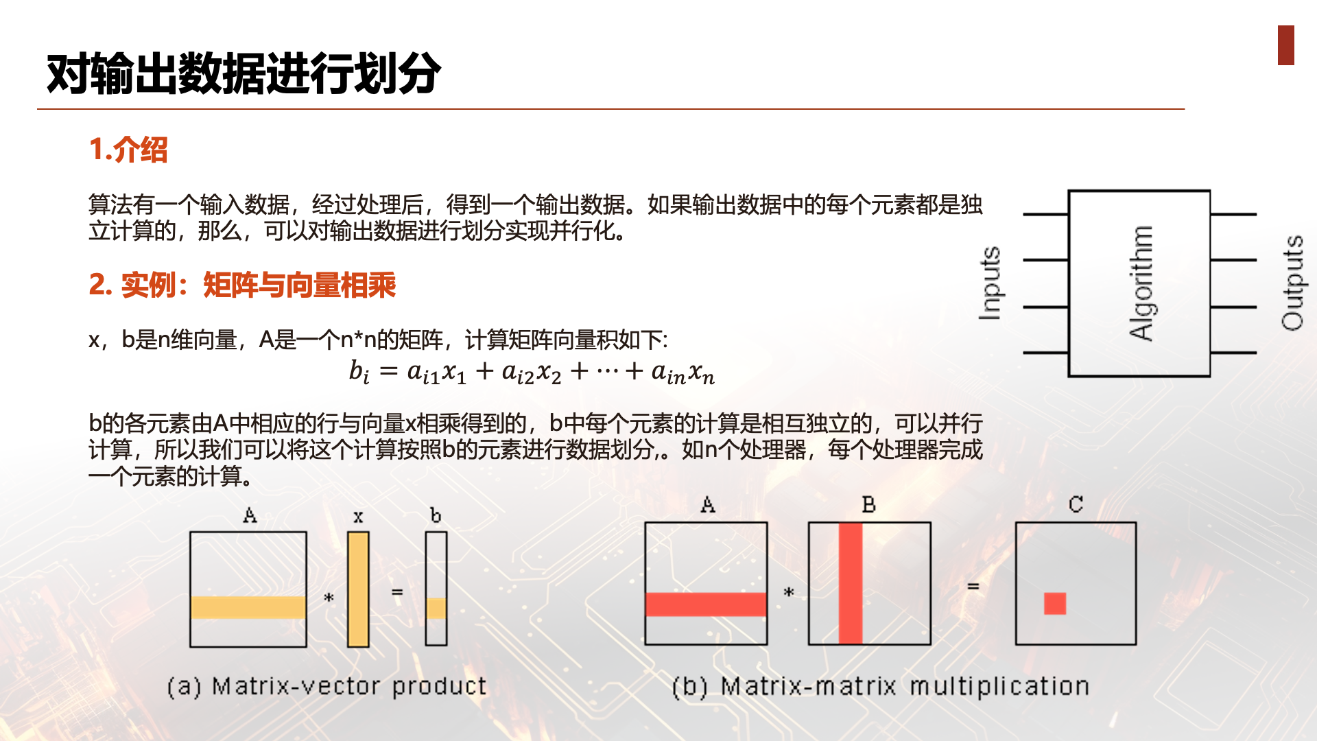
This algorithm has an input set that, after processing, produces an output set. If each element in the output set is computed independently, then any partition of the output set will have a corresponding parallel task decomposition scheme. The maximum parallelism of this decomposition equals the size of the output set. Data decomposition is an effective method for discovering parallelism.

x, b are n-dimensional vectors, and A is an n x n matrix. The matrix-vector product is computed as follows: 　　　　　　　　　　　　　　b=Ax

b is the algorithm's output. Let's see how each element of b is obtained. Each element of b can be obtained by the following formula:

$$b_i = a_{i1}x_1 + a_{i2}x_2 + \cdots + a_{in}x_n$$

Since the computation of each element of b can be done independently (in parallel), we can partition this computation by elements of b: n processors, each computing one element.

Each element of C is the dot product of the i-th row vector of A and the j-th column vector of B. Therefore, data partitioning can be done by elements of C, with the task of computing each element of C as a subtask.

Partitioning Intermediate Data

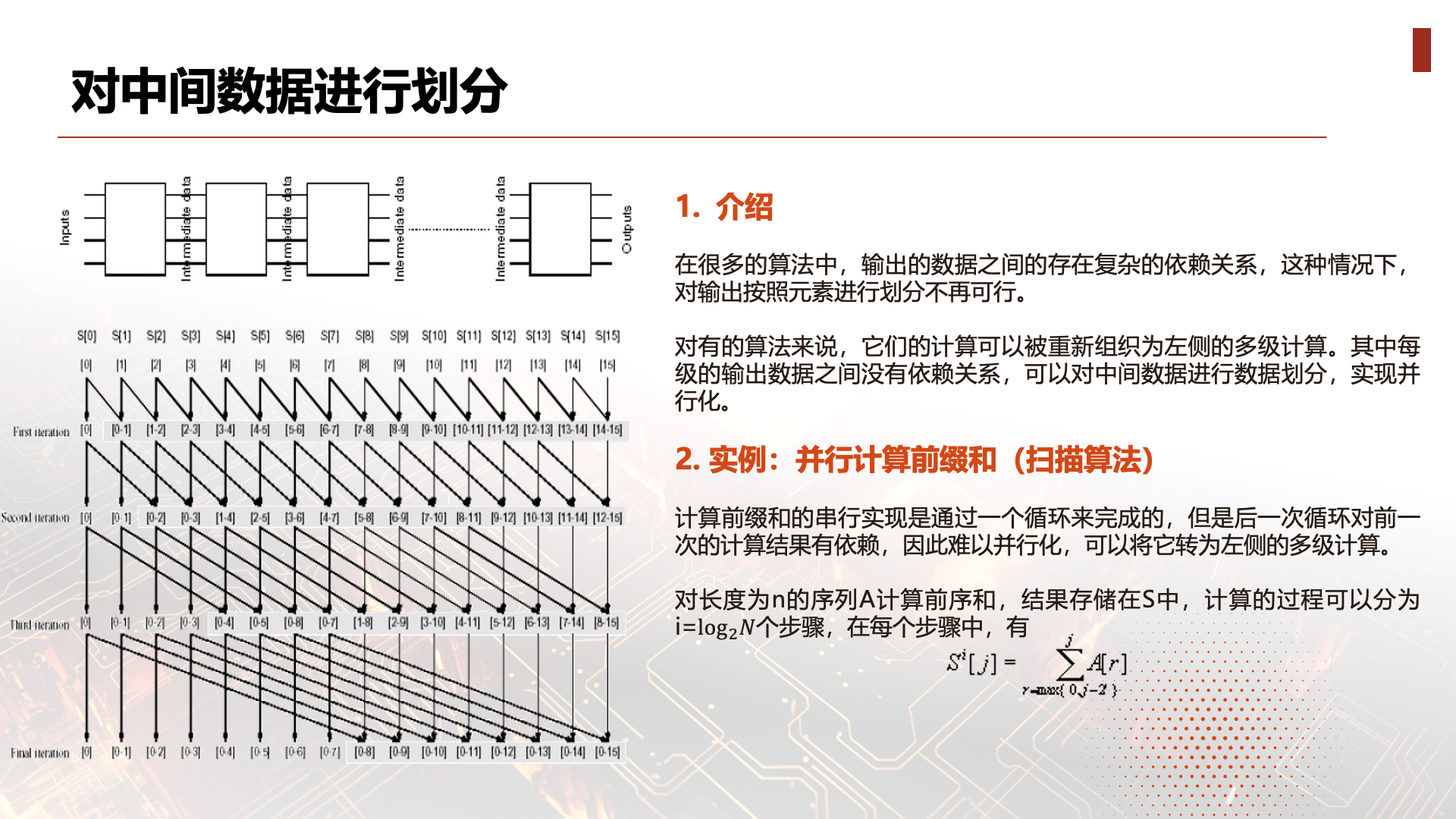
In many algorithms, there are complex dependencies between data in the output set. In such cases, partitioning the output set by element is no longer feasible. For some algorithms, their computations can be reorganized into multi-level computations:

Where the output data at each level has no dependencies (their corresponding computations can be performed in parallel). In this case, data partitioning can be performed on intermediate data (the output of each level).

For example, consider the following prefix sum algorithm:

Computing the prefix sum of a sequence A of length n, storing the result in S. The computation can be divided into i= steps, where in each step, there are .

void hillisSteeleScanParallel(int *input, int *output, int n) {
    // 复制输入到输出，为前缀和计算做准备
    for (int i = 0; i < n; ++i) {
        output[i] = input[i];
    }

    // 对数步骤的Hillis-Steele算法
    for (int step = 1; step < n; step *= 2) {
        // 创建一个临时数组来存储这一步的计算结果
        int *temp = (int *)malloc(n * sizeof(int));
        if (temp == NULL) {
            fprintf(stderr, "Memory allocation failed!\n");
            exit(EXIT_FAILURE);
        }

        // 并行执行每一步的计算
        #pragma omp parallel for
        for (int i = 0; i < n; ++i) {
            if (i < step) {
                temp[i] = output[i];
            } else {
                temp[i] = output[i] + output[i - step];
            }
        }

        // 将临时数组复制回输出数组
        for (int i = 0; i < n; ++i) {
            output[i] = temp[i];
        }

        // 释放临时数组的内存
        free(temp);
    }
}

Partitioning Input Data

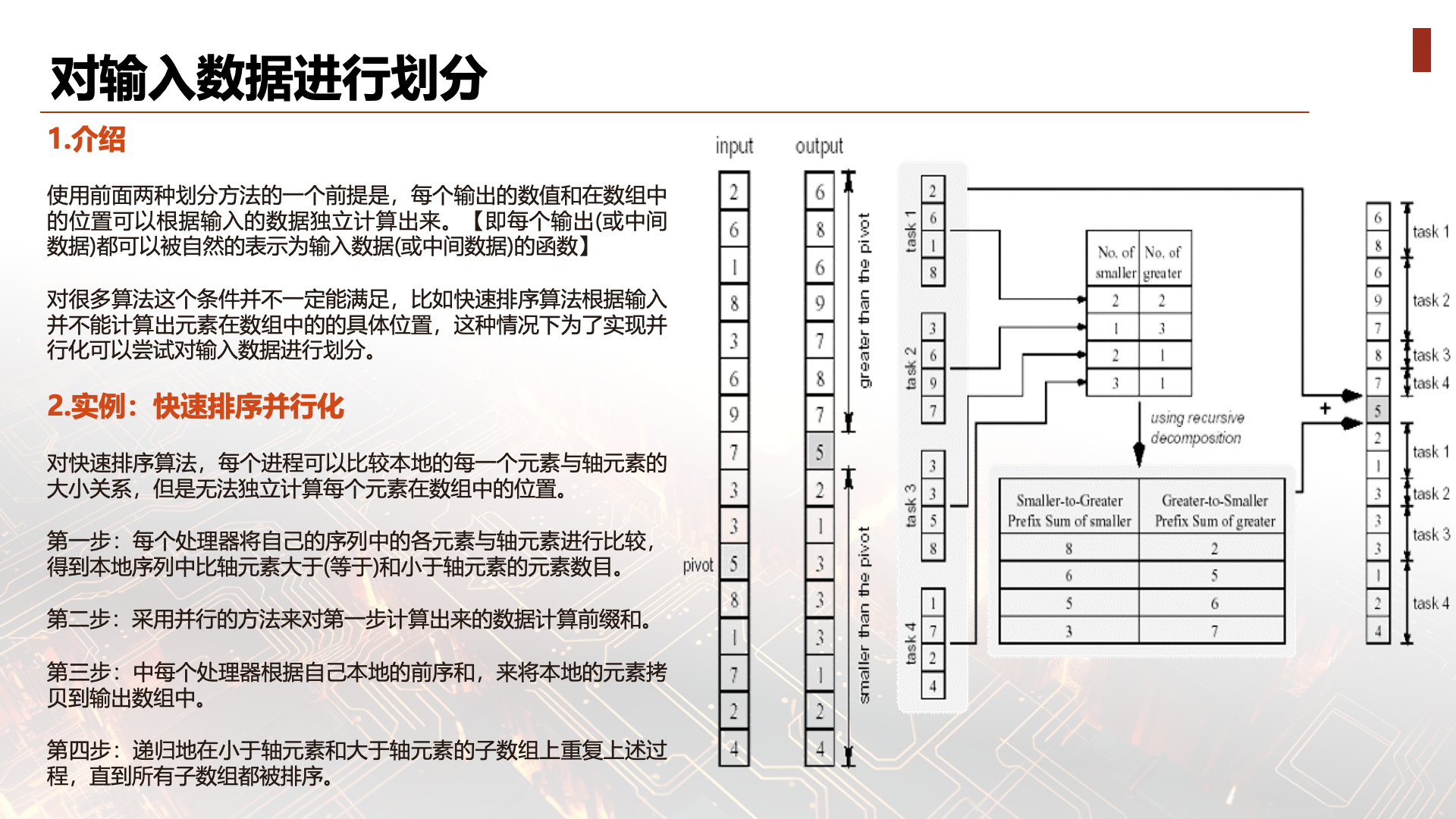
　　The two data partitioning methods discussed above are actually partitioning output data. A prerequisite for being able to perform this partitioning is that each output can be naturally expressed as a function of the input data. For many algorithms, this condition may not be met. For example, for a sorting algorithm, the position of each output element cannot be (efficiently) determined independently. In such cases, since output data cannot be partitioned, one can try to partition the input data instead, and then obtain the parallel task set based on this partition. Each parallel subtask performs as much computation as possible on its own data (or local data). Note that the computation results given by these parallel task sets may not yet be the answer to the original problem. Therefore, an additional computation phase is often needed to generate the final answer from these results.

　　Consider the quicksort algorithm discussed earlier. An important step in the quicksort algorithm is selecting an element from a sequence as the pivot element, then partitioning the sequence so that one subsequence contains all elements smaller than the pivot, and the other subsequence contains elements larger than (or equal to) the pivot. Now consider how to complete this step. Suppose the sequence is an array of n elements. To simplify the discussion, we assume the selected pivot element is unique in the array (i.e., its value is different from all other array elements). The following diagram gives an example (n=16). 5 is selected as the pivot element (the algorithm used for this selection is not discussed here). The left side is the algorithm input, and the right side is the algorithm output (both a single array). Now consider the solution to this problem. To obtain the result sequence, each element of the input array needs to be (independently) compared with the pivot element. Then the number of elements smaller than the pivot and the number of elements larger than the pivot need to be computed. This determines the position (array index) of the pivot element in the output array. The remaining elements can be simply copied from the input array to the output array.

　　The above algorithm cannot use output data partitioning: because the index of each element in the output sequence cannot be independently computed from the input sequence (note: it may be possible, but not efficient). However, this algorithm can develop parallelism through input data partitioning. The details of this partitioning can be seen in the diagram below. An array of 16 elements is evenly divided into 4 subsequences (for assignment to 4 processors for parallel processing).

　　The algorithm includes three phases. In the first phase, each processor compares elements in its own sequence with the pivot element to get the number of elements smaller than the pivot and the number greater than or equal to the pivot in the local sequence. In the second phase, recursive decomposition is used to compute prefix sums of the above data (note that the directions for counting small and large elements are different). In the third phase, each processor copies its local elements to the output array based on its local prefix sums (which actually give the indices of the output array).

　　For some algorithms, although output data partitioning can be used, partitioning input data on top of that may provide additional parallelization approaches. Consider the following example: computing the frequency of a set of itemsets in a transaction database. Transaction set T contains n transactions, and itemset I contains m sub-itemsets (I = I1, I2, ..., Im). Each transaction and itemset consists of some items, all contained in a possible itemset M. The computation output is the total count of occurrences of each itemset Ii across all transactions. The diagram below gives a computation example.

　　In this example, the database includes 10 transactions, and we are interested in 8 itemsets. The computation result is the total number of occurrences of each itemset in the transactions. For example, itemset {D,E} appears in transactions {B,D,E,F,K,L}, {D,E,F,H}, {D,E,F,K,L}, so its occurrence frequency is 3.

　　Actually, this type of computation is a necessary step in data mining problems, called association rule discovery. The serial algorithm for solving this problem builds a lookup structure (such as a hash tree) for sub-itemsets in I, then for each transaction in T, it enumerates all possible item combinations to see if they match any itemset in I. For example, for transaction {A,B,C}, the algorithm may construct itemsets including {A}, {B}, {C}, {A,B}, {A,C}, {B,C}, {A,B,C} (actually the power set of the transaction minus the empty set), then check if they exist in the lookup structure. If a match is found, the corresponding frequency counter is incremented by 1. The purpose of using a lookup structure is to make the matching process more efficient.

　　In this algorithm, there are two inputs T, I and one output array. They can all be used to partition the algorithm. For example, we can partition T: divide it into two equal-sized subsets, compute each separately, and then assemble the final results. As shown below:

　　Another feasible data partitioning method is to partition the itemset I: divide I into two equal-sized parts, which can independently compute their own frequencies. (Note that the result of partitioning output data is the same as this partitioning, because itemsets and frequencies have a one-to-one correspondence).

Data Partitioning Summary

　　Generally, when we need to decide how to partition data or which data to partition, we need to look at which partitioning gives the best (or simplest) computation partitioning. Because the purpose of data partitioning is only to obtain a reasonable computation partitioning. For some problems, input data partitioning works better, while for others, output data (computation results) partitioning is better. When using data decomposition, all possible data partitioning methods need to be examined.

Owner-Compute Rule

　　The methods introduced above focus on how to partition data and which data to partition. However, since what we need is computation partitioning, how to derive a computation partitioning from a data partitioning is a necessary step in this parallelism development. In fact, all the examples above use an "owner-compute rule" to derive a computation partitioning from a data partitioning. The basic idea is that each computation partition completes all computations for the data it owns. Of course, for different data characteristics and different types of data used for partitioning, the owner-compute rule may have different meanings. For example, when we use input data for partitioning, the owner-compute rule means we perform all computations possible with these (partitioned) input data.而对于输出数据划分，拥有者计算规则则表示生成这些数据所需要的所有计算。

Decomposition Strategies

Decomposition strategies in High-Performance Computing (HPC) typically involve breaking large computational tasks into smaller chunks so they can be executed in parallel on multiple processors to improve computational efficiency. Below are three common decomposition strategies:

Block Decomposition:

Introduction: Block decomposition is typically used for data partitioning, dividing a data set into smaller, equal-sized blocks, with each processor or core processing one or more data blocks.

Applicable scope: Suitable for cases where data can be processed independently, commonly used in matrix operations or image processing. Block Decomposition Example

    int remainder = n % world_size;
    for (int i = 0; i < world_size; i++)
    {
        counts[i] = n / world_size + (i < remainder ? 1 : 0);
        displacements[i] = (i > 0) ? (displacements[i - 1] + counts[i - 1]) : 0;
    }

Cyclic Decomposition:

Introduction: Cyclic decomposition distributes loop iterations to different processors, typically in a round-robin fashion. For example, if there are 4 processors, processor 1 gets all iterations of the form 4n+1, processor 2 gets iterations of the form 4n+2, and so on. Applicable scope: This approach is suitable for scenarios with many iterations but small computation per iteration. Cyclic decomposition is suitable for loops with a large number of independent iterations and relatively uniform computation per iteration, enabling effective load balancing across multiple processors. Cyclic Decomposition Example

    int rank, size;
    MPI_Init(&argc, &argv);
    MPI_Comm_rank(MPI_COMM_WORLD, &rank);
    MPI_Comm_size(MPI_COMM_WORLD, &size);   

		n_iterations = 100; // 假设我们有100次迭代
    // 循环分解
    for (i = rank; i < n_iterations; i += size) {
        // 在这里执行每次迭代的工作
        // rank表示当前进程编号，i表示迭代索引
        printf("Processor %d is doing iteration %d\n", rank, i);
        // ... 进行计算 ...
    }

    MPI_Finalize(); // 结束MPI环境
    return 0;

Block-Cyclic Decomposition:

Introduction: Block-cyclic decomposition is a combination of block decomposition and cyclic decomposition. Data is divided into blocks, but the blocks are assigned to processors in a cyclic manner. This method can both maintain load balancing and reduce communication overhead.

Applicable scope: Suitable for cases where there is significant data exchange between processors.

Block-Cyclic Decomposition Example

    int rank, size;
    MPI_Init(&argc, &argv);
    MPI_Comm_rank(MPI_COMM_WORLD, &rank);
    MPI_Comm_size(MPI_COMM_WORLD, &size); 

int rows_per_process = MATRIX_SIZE / size;  // 每个进程处理的行数
    int remaining_rows = MATRIX_SIZE % size;    // 剩余的行数

    // 分配额外的行
    if (rank < remaining_rows) {
        rows_per_process++;
    }

    for (int block_start = 0; block_start < rows_per_process; block_start += BLOCK_SIZE) {

        // 处理当前块
        process_block(start_row, end_row, rank);
    }

Other Knowledge Points

void* Automatic Data Type Conversion

In C, the return type of the malloc function is void*, which is a generic pointer type that can be converted to any other pointer type without losing information. In the C standard, a void* pointer can be automatically and implicitly converted to other pointer types.

Therefore, in C, the following code:

int *counts = malloc(sizeof(int) * world_size);

is perfectly valid, because the returned void* pointer is automatically converted to an int* pointer. The compiler performs this conversion at compile time, without needing an explicit type cast.

However, in C++, this implicit conversion is not allowed. If you use malloc in C++ code, you need to explicitly cast:

int *counts = (int *)malloc(sizeof(int) * world_size);

But in C++, it is generally not recommended to use malloc and free. Instead, it is recommended to use the new and delete operators, because they support constructor and destructor calls, which malloc and free do not.

Overall, in C, your code is fine and does not need explicit casting. However, if your code needs to be compiled in a C++ environment, you need to add a type cast, or better yet, use C++ memory allocation methods.

When does automatic data type conversion occur?

In C, void* pointers can be automatically converted to any other pointer type. This conversion is implicit and does not require the programmer to explicitly perform a type cast. This is a feature of C that allows flexible pointer operations.

Here are several cases where void* pointers are automatically converted:

1. Assignment to other pointer types: When you assign a void* pointer to another pointer type, the conversion is automatic.

   void* vptr = ...;
   int* iptr = vptr; // 自动转换为 int* 类型

2. As a function parameter: When you pass a void* pointer to a function parameter that accepts a specific pointer type, the conversion is also automatic.

   void some_function(int* ptr);
   
   void* vptr = ...;
   some_function(vptr); // 自动转换为 int* 类型

3. Returning from a function: If the function return type is a non-void* pointer type, then returning a void* pointer from the function also triggers automatic conversion.

   int* some_function() {
       void* vptr = ...;
       return vptr; // 自动转换为 int* 类型
   }

However, explicit conversion is needed in the following cases:

1. When the compiler needs type information: For example, when you need to access struct members through a pointer, you must cast the void* pointer to the correct type.

   typedef struct {
       int a;
   } MyStruct;
   
   void* vptr = ...;
   int value = ((MyStruct*)vptr)->a; // 需要显式转换来访问成员

2. In C++: In C++, void* pointers do not automatically convert to other pointer types; explicit casting is required.

   void* vptr = ...;
   int* iptr = static_cast<int*>(vptr); // C++ 需要显式转换

3. In cases involving pointer arithmetic: void* pointers cannot be directly used for pointer arithmetic because the size of the void type is undefined. In such cases, you need to cast void* to another pointer type, such as char*, because char has a defined size (1 byte).

   void* vptr = ...;
   vptr = (char*)vptr + 1; // 需要显式转换为 char* 来进行指针算术

In C, you generally do not need to explicitly cast from void* to other pointer types, unless you are performing operations that require knowing the specific size or type information of the data the pointer points to. In C++, you always need to perform explicit casting.