Ding Zhiyu Week 5 Study Report

[TOC]

Matrix Knowledge

Matrix-Vector Multiplication

Matrix-vector multiplication is one of the fundamental operations in linear algebra, following specific rules. In mathematics, a matrix can be viewed as a linear transformation, and a vector can be viewed as a point or arrow in space. When we multiply a matrix by a vector, we are essentially applying this linear transformation to the vector.

Rules for Matrix-Vector Multiplication

Suppose we have an $m \times n$ matrix $A$ and an $n$-dimensional column vector $\mathbf{x}$. Their product is an $m$-dimensional column vector $\mathbf{y}$. This product is defined as:

$$A\mathbf{x} = \mathbf{y}$$

Where $A$ is such a matrix:

$$A = \begin{bmatrix} a_{11} & a_{12} & \cdots & a_{1n} \\ a_{21} & a_{22} & \cdots & a_{2n} \\ \vdots & \vdots & \ddots & \vdots \\ a_{m1} & a_{m2} & \cdots & a_{mn} \end{bmatrix}$$

$\mathbf{x}$ is such a vector:

$$\mathbf{x} = \begin{bmatrix} x_{1} \\ x_{2} \\ \vdots \\ x_{n} \end{bmatrix}$$

Then each element $y_i$ of the product $\mathbf{y}$ ($i$ from 1 to $m$) can be computed as:

$$y_i = a_{i1}x_1 + a_{i2}x_2 + \cdots + a_{in}x_n$$

Or more compactly:

$$y_i = \sum_{j=1}^{n} a_{ij}x_j$$

Example

Suppose we have a $2 \times 3$ matrix $A$ and a $3$-dimensional column vector $\mathbf{x}$:

$$A = \begin{bmatrix} 2 & 0 & 1 \\ -1 & 3 & 4 \end{bmatrix}, \quad \mathbf{x} = \begin{bmatrix} 3 \\ 5 \\ 1 \end{bmatrix}$$

Then their product $\mathbf{y}$ will be:

$$\mathbf{y} = A\mathbf{x} = \begin{bmatrix} 2 & 0 & 1 \\ -1 & 3 & 4 \end{bmatrix} \begin{bmatrix} 3 \\ 5 \\ 1 \end{bmatrix} = \begin{bmatrix} (2 \cdot 3) + (0 \cdot 5) + (1 \cdot 1) \\ (-1 \cdot 3) + (3 \cdot 5) + (4 \cdot 1) \end{bmatrix} = \begin{bmatrix} 7 \\ 14 \end{bmatrix}$$

Here we computed the values of $y_1$ and $y_2$ respectively:

• For $y_1$, we computed $2 \cdot 3 + 0 \cdot 5 + 1 \cdot 1 = 7$
• For $y_2$, we computed $-1 \cdot 3 + 3 \cdot 5 + 4 \cdot 1 = 14$

Notes

• The number of columns of matrix $A$ must equal the number of rows of vector $\mathbf{x}$.
• The dimension of the result $\mathbf{y}$ will be the same as the number of rows of matrix $A$.
• Matrix-vector multiplication is not commutative, i.e., $A\mathbf{x} \neq \mathbf{x}A$.
• Matrix-vector multiplication is distributive and associative, i.e., $A(\mathbf{x} + \mathbf{y}) = A\mathbf{x} + A\mathbf{y}$, and $(AB)\mathbf{x} = A(B\mathbf{x})$, where $A$ and $B$ are matrices and $\mathbf{x}$ and $\mathbf{y}$ are vectors.

Matrix-vector multiplication is very important in many fields, including computer graphics, engineering, physics, statistics, and machine learning/data science, among others.

Matrix Multiplication

Matrix multiplication involves multiplying the rows of the first matrix by the columns of the second matrix. Each row is multiplied by each column.

The number of rows in the result is determined by the first matrix, and the number of columns is determined by the second matrix.

Matrix multiplication is a core concept in linear algebra, used to combine information from two matrices. Suppose we have two matrices $A$ and $B$, and their product is a third matrix $C$. The definition of matrix multiplication is as follows:

• Matrix $A$ has size $m \times n$, meaning it has $m$ rows and $n$ columns.
• Matrix $B$ has size $n \times p$, meaning it has $n$ rows and $p$ columns.
• To perform the multiplication, the number of columns of matrix $A$ must equal the number of rows of matrix $B$.

If the above conditions are met, then the product of matrix $A$ and matrix $B$ is an $m \times p$ matrix $C$. Each element $c_{ij}$ of matrix $C$ is obtained by multiplying the corresponding elements of the $i$-th row of matrix $A$ with the $j$-th column of matrix $B$ and summing them:

$$c_{ij} = a_{i1}b_{1j} + a_{i2}b_{2j} + \cdots + a_{in}b_{nj} = \sum_{k=1}^{n} a_{ik}b_{kj}$$

Where $i = 1, 2, \ldots, m$ and $j = 1, 2, \ldots, p$.

Example

Let's illustrate how matrix multiplication works with a concrete example:

Suppose we have the following two matrices $A$ and $B$:

$$A = \begin{bmatrix} 2 & 0 \\ -1 & 3 \end{bmatrix}, \quad B = \begin{bmatrix} 1 & 4 \\ 2 & -1 \end{bmatrix}$$

Matrix $A$ is a $2 \times 2$ matrix, and matrix $B$ is also a $2 \times 2$ matrix. Their product $C$ will be:

$$C = AB = \begin{bmatrix} (2 \cdot 1 + 0 \cdot 2) & (2 \cdot 4 + 0 \cdot -1) \\ (-1 \cdot 1 + 3 \cdot 2) & (-1 \cdot 4 + 3 \cdot -1) \end{bmatrix} = \begin{bmatrix} 2 & 8 \\ 5 & -7 \end{bmatrix}$$

Here, each element of $C$ is computed as follows:

• $c_{11} = (2 \cdot 1) + (0 \cdot 2) = 2$
• $c_{12} = (2 \cdot 4) + (0 \cdot -1) = 8$
• $c_{21} = (-1 \cdot 1) + (3 \cdot 2) = 5$
• $c_{22} = (-1 \cdot 4) + (3 \cdot -1) = -7$

Notes

• Matrix multiplication is not commutative, i.e., $AB \neq BA$ in general.
• Matrix multiplication is associative, i.e., $(AB)C = A(BC)$.
• Matrix multiplication is distributive, i.e., $A(B + C) = AB + AC$.
• Matrix multiplication typically involves a large number of multiplication and addition operations, so it can be computationally expensive, especially for large matrices.

Matrix multiplication has wide applications in many fields, including data processing, physical sciences, engineering, computer graphics, and economics, among others.

Now, let's implement matrix multiplication in C. Below is a simple program that implements the multiplication of two matrices:

#include <stdio.h>

#define MAX_SIZE 100

void matrixMultiply(int m, int n, int p, int A[][MAX_SIZE], int B[][MAX_SIZE], int C[][MAX_SIZE]) {
    for (int i = 0; i < m; i++) {
        for (int j = 0; j < p; j++) {
            C[i][j] = 0; // 初始化结果矩阵的当前元素为0
            for (int k = 0; k < n; k++) {
                C[i][j] += A[i][k] * B[k][j]; // 计算结果矩阵的当前元素
            }
        }
    }
}

int main() {
    int m, n, p;
    int A[MAX_SIZE][MAX_SIZE], B[MAX_SIZE][MAX_SIZE], C[MAX_SIZE][MAX_SIZE];

    // 假设用户将输入矩阵的大小和元素
    printf("Enter rows and columns for matrix A: ");
    scanf("%d %d", &m, &n);

    printf("Enter elements of matrix A:\n");
    for (int i = 0; i < m; i++)
        for (int j = 0; j < n; j++)
            scanf("%d", &A[i][j]);

    printf("Enter rows and columns for matrix B: ");
    scanf("%d %d", &n, &p); // 注意：这里n应该与之前输入的n相同

    printf("Enter elements of matrix B:\n");
    for (int i = 0; i < n; i++)
        for (int j = 0; j < p; j++)
            scanf("%d", &B[i][j]);

    // 执行矩阵乘法
    matrixMultiply(m, n, p, A, B, C);

    // 打印结果矩阵
    printf("Result of matrix multiplication:\n");
    for (int i = 0; i < m; i++) {
        for (int j = 0; j < p; j++)
            printf("%d ", C[i][j]);
        printf("\n");
    }

    return 0;
}

This program first defines a matrixMultiply function that accepts the dimensions and elements of two matrices and then computes their product. The main function is used to get the matrix dimensions and elements from user input, call the matrixMultiply function to compute the product, and finally print the result matrix.

Note that this program assumes the user will enter valid matrix dimensions, where the number of columns of matrix A equals the number of rows of matrix B, and all matrix dimensions do not exceed the size defined by MAX_SIZE. In practice, you may need to add additional error checking to ensure input validity.

Practice: Parallelizing Matrix Multiplication with MPI

The code is in the Matrix_MPI folder.

Problems Encountered in the First Matrix Parallelization

Some issues in the code are as follows:

1. The case where the matrix size is not evenly divisible among processes is not handled. In the A_local_row = m / size; calculation, if m is not divisible by size, it will result in uneven row distribution.

2. The MPI_Gather call may be incorrect. If m is not divisible by size, the last process may have a different number of rows, requiring MPI_Gatherv to handle different receive counts.

3. MPI_Scatter and MPI_Gather use the A and C arrays, but these arrays are uninitialized in non-root processes.

4. The max_elapsed_time in the MPI_Reduce call is only declared inside the rank == 0 block, which will cause a compilation error because it is undeclared in other processes.

N-Body Problem

Introduction

In parallel programming and computational physics, the n-body problem typically refers to simulating and computing the dynamics of a system composed of n interacting particles. In astrophysics, these particles can be stars, planets, or other celestial bodies that interact through gravitational forces; in molecular dynamics, particles can be atoms or molecules that interact through electromagnetic forces. The goal of the n-body problem is to determine the motion of all particles in the system over time.

The n-body problem is a classic physics problem because it involves nonlinear multi-body interactions, making analytical solutions usually impossible except for very simple cases (such as the two-body problem). Therefore, scientists typically use numerical methods to approximately solve the n-body problem, which involves iteratively computing particle positions and velocities through discrete time steps.

Parallel programming is very important in solving the n-body problem because:

1. Large computational load: The computational complexity of the n-body problem grows significantly with the number of particles. At each time step, each particle needs to compute interaction forces with all other particles, leading to quadratic growth in computation as the number of particles increases.

2. Divisibility: The computation of the n-body problem can be naturally divided into multiple tasks, each computing the interaction forces for a subset of particles, making it very suitable for parallel processing.

3. Real-time requirements: In some applications, such as video games or real-world simulations, the solution to the n-body problem needs to be computed in real-time or near real-time, and parallel processing can provide sufficient computational resources to meet these requirements.

Parallel solutions to the n-body problem typically involve the following steps:

• Task decomposition: Divide the entire problem into smaller tasks that can be processed in parallel.
• Compute interactions: Compute the interaction forces between each pair of particles in parallel.
• Integrate results: Merge the results of parallel computations to update each particle's position and velocity.
• Time advancement: Advance the system by one time step and repeat the above process.

Methods for implementing parallel computation include using multi-threading, multi-processors, multi-core CPUs, and graphics processing units (GPUs), among other technologies. GPUs, in particular, are very suitable for handling this type of computationally intensive task due to their large number of parallel processing units.

In programming practice, parallel algorithms for solving the n-body problem need to be carefully designed to minimize communication overhead between processes or threads and maximize the overlap of computation with communication to improve parallel efficiency.

Basic Physics Knowledge in the N-Body Problem

1. Universal Law of Gravitation

   Newton's universal law of gravitation describes the gravitational force between two objects. Its magnitude is proportional to the product of the two objects' masses and inversely proportional to the square of the distance between them. The formula is:

   $F = G \frac{m_1 m_2}{r^2}$

   Where:

   • $F$ is the gravitational force between the two objects.
   • $G$ is the gravitational constant, approximately $6.67430 \times 10^{-11} \text{m}^3\text{kg}^{-1}\text{s}^{-2}$.
   • $m_1$ and $m_2$ are the masses of the two objects.
   • $r$ is the distance between the two objects.

2. Newton's Laws of Motion

   Newton's second law of motion describes the relationship between force and the change in an object's state of motion, i.e., force equals mass times acceleration:

   $F = m a$

   Where:

   • $F$ is the net force acting on the object.
   • $m$ is the mass of the object.
   • $a$ is the acceleration of the object.

3. Computing Gravitational Force

   The gravitational_force function in the code implements the computation of the universal law of gravitation. First, it computes the distance between two objects:

   $\text{distance} = \sqrt{(x_2 - x_1)^2 + (y_2 - y_1)^2 + (z_2 - z_1)^2}$

   Then, based on the universal law of gravitation, it computes the magnitude of the gravitational force, and finally decomposes this force along three coordinate axes to obtain the force in vector form.

4. Updating Velocity and Position

   In the update_bodies function, the net force on each object is first computed, and then the object's velocity is updated according to Newton's second law of motion:

   $v_{\text{new}} = v_{\text{old}} + \frac{F}{m} \Delta t$

   Where $\Delta t$ is the time step.

   Finally, the object's position is updated, assuming velocity is constant over the small time step $\Delta t$:

   $x_{\text{new}} = x_{\text{old}} + v \Delta t$

   This simple update method is called the Euler method. It may not be very stable or accurate numerically, especially with larger time steps or in complex dynamical systems. For more complex or higher-precision systems, more advanced integration methods such as the Runge-Kutta method may be needed.

5. Simulation Loop In the main function, there is a simulation loop that repeatedly calls the update_bodies function to simulate the motion of objects over time. Each loop iteration represents time advancing by $\Delta t$.

Notes

In actual numerical simulations, factors such as numerical stability and energy conservation also need to be considered. For example, when objects are very close together, the above method may lead to numerical instability because the gravitational force becomes very large. Additionally, the Euler method may cause energy to gradually increase or decrease over long integration periods, which is physically incorrect. To address these issues, higher-order integration methods can be used, or a softening length can be introduced to prevent the gravitational force from becoming infinite when objects are very close together.

Practice: Parallelizing the N-Body Problem with MPI

The code is in the N_Body_Problem folder.

Knowledge Points

Special Usage of MPI_Allgather (MPI_IN_PLACE)

In MPI, MPI_Allgather is a collective communication operation used to collect data among all participating processes and distribute the collected data to all processes. This function is typically used when each process has a data block and wants every process to receive all other processes' data blocks.

The function prototype is:

int MPI_Allgather(const void *sendbuf, int sendcount, MPI_Datatype sendtype,
                  void *recvbuf, int recvcount, MPI_Datatype recvtype, MPI_Comm comm)

Parameter descriptions:

• sendbuf: Pointer to the start of the send buffer, i.e., the memory address containing data to be sent.
• sendcount: Number of data elements to be sent.
• sendtype: MPI data type of the data to be sent.
• recvbuf: Pointer to the start of the receive buffer, i.e., the memory address for storing data sent by all processes.
• recvcount: Number of data elements to be received from each process.
• recvtype: MPI data type of the data to be received.
• comm: MPI communicator, typically MPI_COMM_WORLD, which includes all processes.

In the code snippet you provided:

MPI_Allgather(MPI_IN_PLACE, local_n * sizeof(Vector3D), MPI_BYTE,
              positions, local_n * sizeof(Vector3D), MPI_BYTE, MPI_COMM_WORLD);

Parameter descriptions are as follows:

• MPI_IN_PLACE: This is a special parameter that tells the MPI function to perform the operation in-place. When using MPI_IN_PLACE, the input data (send buffer) and output data (receive buffer) use the same buffer. This means each process's send buffer is its corresponding position in the receive buffer. Using MPI_IN_PLACE can avoid unnecessary data copying and improve efficiency.
• local_n * sizeof(Vector3D): This specifies the amount of data each process sends, i.e., the total number of bytes in each process's local arrays local_positions and local_velocities. Here local_n is the number of Vector3D elements each process is responsible for, and sizeof(Vector3D) is the size of a Vector3D structure (in bytes).
• MPI_BYTE: This is a basic MPI data type indicating that data will be sent and received in bytes. This means MPI will not interpret the actual structure of the data, simply transmitting bytes.
• positions: This is the receive buffer where data from all processes will be collected and stored.
• local_n * sizeof(Vector3D): This specifies the amount of data each process receives, i.e., the size of each process's segment in the positions array.
• MPI_COMM_WORLD: This is a communicator that includes all MPI processes.

So, the purpose of this line of code is: each process sends its local_n Vector3D structures and collects the same amount and type of data from other processes, storing the result in the positions array. Because MPI_IN_PLACE is used, both sending and receiving are performed on the positions array, requiring no additional send buffer. This way, after executing this operation, each process will have the complete position information of the entire system.

Is it correct to place MPI_IN_PLACE in the receive buffer position?

No, such code is incorrect. In the MPI_Allgather call, when using MPI_IN_PLACE, it should only appear in the send buffer (sendbuf) position, and the receive buffer (recvbuf) should be a different buffer for receiving data from all processes. MPI_IN_PLACE is used to indicate to the MPI library that the sending data is already in the corresponding position of the receive buffer, so no separate send buffer is needed.

The correct MPI_Allgather call using MPI_IN_PLACE should look like this:

MPI_Allgather(MPI_IN_PLACE, 0, MPI_DATATYPE_NULL,
              positions, local_n * sizeof(Vector3D), MPI_BYTE, MPI_COMM_WORLD);

Here, MPI_IN_PLACE tells the MPI library to collect data in-place, i.e., operating directly in the positions array. Since we are operating in-place, the send count (sendcount) and send type (sendtype) will not be used, so sendcount can be set to 0 and sendtype can be set to MPI_DATATYPE_NULL.

In the code you provided:

MPI_Allgather(positions, local_n * sizeof(Vector3D), MPI_BYTE,
              MPI_IN_PLACE, local_n * sizeof(Vector3D), MPI_BYTE, MPI_COMM_WORLD);

If you try to use MPI_IN_PLACE in the receive buffer position, it will cause an error because MPI_IN_PLACE is specifically designed for the send buffer position to inform the MPI library that sending and receiving use the same buffer. Furthermore, the positions of the send buffer (sendbuf) and receive buffer (recvbuf) cannot be swapped. The correct usage is to place MPI_IN_PLACE in the sendbuf position and provide an appropriate receive buffer.

Multi-dimensional Array Parameter Passing

The first dimension can be omitted, but other dimensions cannot, because the compiler needs to know the number of elements in each dimension to perform indexing on a one-dimensional array.

In C, when passing a multi-dimensional array as a function parameter, the size of all dimensions except the first must be specified. This is because the compiler needs this information to calculate the position of array elements.

For a one-dimensional array, when passing it as a parameter to a function, what is actually passed is a pointer to the first element. Therefore, the length of a one-dimensional array is usually optional in function parameters, e.g., int vector[] or int *vector.

However, for a multi-dimensional array, you must specify the other dimensions besides the first so the compiler can correctly calculate offsets. For example, if you have a two-dimensional array int matrix[3][3] and want to pass it to a function, your function parameter should specify the size of the second dimension, such as int matrix[][3].

In the example I gave earlier, N is a preprocessor macro that defines the array size. Therefore, when you see int matrix[N][N] as a function parameter, it means N must be defined before the function is called.

Here is a modified matrixVectorMultiply function that uses the correct parameter declaration:

void matrixVectorMultiply(int matrix[][N], int vector[N], int result[N]);

Here, we specify that the second dimension of matrix is N, while vector and result as one-dimensional arrays have optional sizes. However, for clarity and readability, I included the size N in the previous example. If you don't need to know the size of a one-dimensional array in the function implementation, you can choose to omit it, as follows:

void matrixVectorMultiply(int matrix[][N], int vector[], int result[]);

In this case, you need to ensure that arrays of the correct size are passed when the function is called.

Choosing Between Three Point-to-Point Communication Methods

The best time to use blocking, buffered, or non-blocking communication usually depends on the specific requirements of the application, communication patterns, and performance goals. Below are some guidelines to help you decide:

Blocking Communication (MPI_Send, MPI_Recv)

• Simplicity: If your program logic is simple and you don't need to perform computation and communication simultaneously, standard blocking communication may be the simplest choice.
• Determinism: When you need to ensure that a message has been sent or received before executing subsequent code, blocking communication provides this certainty.
• Small messages: For small messages, the overhead of blocking communication may be negligible, as small messages are usually sent or received very quickly.

Buffered Send (MPI_Bsend)

• Available buffer: If your system has sufficient buffer resources and you want to avoid potential blocking in send operations, buffered send can be a good choice.
• Medium-sized messages: For medium-sized messages, using buffered send can reduce blocking time in send operations, as data is copied to a buffer.
• Overlap computation with communication: If you want to perform some computation while messages are being sent, buffered send can provide this overlap possibility, although it is not as flexible as non-blocking communication.

Non-blocking Communication (MPI_Isend, MPI_Irecv)

• Performance: When you need to maximize program performance, especially when computation and communication overlap is needed, non-blocking communication is usually the preferred choice.
• Large messages: For large messages, non-blocking communication allows the send operation to perform other computations during data transfer, improving resource utilization.
• Complex communication patterns: In programs with complex communication patterns, non-blocking communication can provide better control, as it allows initiating multiple communication operations simultaneously and processing them as they complete.
• Pipeline operations: If your application can be divided into multiple stages that can be processed in parallel, non-blocking communication can help you set up pipelines where computation and communication can execute in parallel across different stages.

Summary

• If your application has a simple communication pattern, or you are just starting to use MPI, then starting with standard blocking communication is reasonable.
• If your application needs to perform some computation during communication and you don't want to deal with the complexity of non-blocking communication, buffered send may be a good intermediate choice.
• If you need to maximize performance, especially with a large amount of concurrent communication and computation, then non-blocking communication is the best choice.

In any case, the best approach is to determine which communication method is most suitable for your application through experimentation and performance analysis. Different hardware and network architectures may also affect the best choice.

Buffered Send MPI_Bsend Function

The MPI_Bsend function is a buffered send function with the following prototype:

int MPI_Bsend(const void *buf, int count, MPI_Datatype datatype, int dest, int tag, MPI_Comm comm)

Below is a detailed explanation of each parameter:

• const void *buf: This is a pointer to the starting position of the message to be sent. This buffer contains the data to be sent.

• int count: This parameter specifies the number of data elements to be sent. Combined with the data type (datatype), this parameter defines the total size of data in the send buffer.

• MPI_Datatype datatype: This parameter specifies the data type of each data element. MPI predefines a series of data types, such as MPI_INT for integers, MPI_FLOAT for floating-point numbers, etc.

• int dest: This parameter specifies the rank (identifier) of the destination process. In MPI, each process has a unique rank used to identify the target or source of communication.

• int tag: This parameter is an integer tag used to distinguish different messages. The tags in send and receive operations must match to correctly pair messages.

• MPI_Comm comm: This parameter specifies the communicator, which is a context for a group of processes that can communicate with each other. The most commonly used communicator is MPI_COMM_WORLD, which includes all MPI processes.

Regarding buffer allocation, you need to manually allocate the buffer before calling MPI_Bsend. The buffer size should be large enough to accommodate all outbound messages plus any additional overhead that the MPI library may need. MPI defines a constant MPI_BSEND_OVERHEAD that represents the additional overhead that each buffered send operation may require.

Below is example code for allocating and attaching a buffer:

int buffer_size = messages_count * (message_size + MPI_BSEND_OVERHEAD);
void* buffer = malloc(buffer_size);

// 附加缓冲区
MPI_Buffer_attach(buffer, buffer_size);

// ... 进行缓冲发送操作 ...

// 分离缓冲区
void* bsend_buff;
int bsend_size;
MPI_Buffer_detach(&bsend_buff, &bsend_size);

// 释放缓冲区内存
free(buffer);

In this example, messages_count is the number of messages you intend to send, and message_size is the size of a single message. This size should be determined based on the maximum message size to be sent in the actual application. Note that the MPI_Buffer_attach function requires the buffer size (in bytes), including MPI_BSEND_OVERHEAD for each message. When the buffer is no longer needed, use MPI_Buffer_detach to detach the buffer and release the buffer memory at the appropriate time.

Differences in Resource Usage Between Non-blocking Communication and Buffered Send

Non-blocking communication and buffered send (such as MPI_Bsend in MPI) have some differences in resource usage, but this does not mean that non-blocking communication always consumes more buffer resources. In fact, their respective resource usage depends on various factors, including the communication library implementation, system configuration, and communication patterns.

The buffer is divided into two: a send buffer and a user-pre-allocated buffer. Isend sends from the send buffer, while Bsend copies data from the send buffer to the user-pre-allocated buffer and then sends it. After the function returns, you can immediately change the data in the send buffer because there is a copy in the user-pre-allocated buffer that won't affect the sending.

Non-blocking communication:

• Non-blocking communication operations (such as MPI_Isend and MPI_Irecv) allow the program to continue executing other operations while waiting for data transfer to complete.
• Non-blocking communication may require additional state tracking resources because the communication library needs to record the progress of operations to be able to retrieve status when checking or waiting later.
• In non-blocking communication, data may be copied to an internal buffer or sent directly from the user-provided buffer, depending on the communication library implementation and message size.

Buffered send:

• Buffered send (such as MPI_Bsend) requires the user to pre-allocate a sufficiently large buffer. The MPI library uses this buffer to store messages about to be sent.
• Once a message is copied to this buffer, the send operation can return, while the actual transfer may occur later.
• The advantage of buffered send is that once a message is copied to the buffer, the send buffer can be immediately reused without waiting for the message to actually be sent to the receiver.
• Buffered send may consume more user-space memory because sufficient space must be allocated for the buffer to store all outbound messages.

In some cases, non-blocking communication may be more efficient than buffered send because it can reduce buffer requirements, especially when the communication library can use the underlying hardware's direct memory access (DMA) capabilities for data transfer. However, in other cases, if non-blocking communication requires frequent copying of data to internal buffers, it may use more buffer resources.

Overall, non-blocking communication and buffered send each have their advantages and disadvantages. Their differences in resource usage depend on specific usage scenarios and MPI implementation details. Generally, the choice of communication method should be based on understanding the application's performance requirements and resource constraints.

Blocking Communication Example

First, let's look at a simplified matrix-vector multiplication example using blocking communication. In this example, we assume the matrix has been divided by rows and distributed to each process.

#include <mpi.h>
#include <stdio.h>
#include <stdlib.h>

int main(int argc, char** argv) {
    int rank, size;
    MPI_Init(&argc, &argv);
    MPI_Comm_rank(MPI_COMM_WORLD, &rank);
    MPI_Comm_size(MPI_COMM_WORLD, &size);

    // 假设n是全局大小，local_n是每个进程的局部大小
    int n = 4; // 举例，全局大小为4
    int local_n = n / size; // 假设能够整除

    // 分配内存
    double A[local_n][n], x[n], y[local_n];

    // 初始化A和x
    // ...

    // 分发向量x中的元素到所有进程
    for (int i = 0; i < size; ++i) {
        if (rank == i) {
            // 主进程发送x的部分到所有其他进程
            for (int j = 0; j < size; ++j) {
                if (j != i) {
                    MPI_Send(x + i * local_n, local_n, MPI_DOUBLE, j, 0, MPI_COMM_WORLD);
                }
            }
        } else {
            // 非主进程接收x的部分
            MPI_Recv(x + i * local_n, local_n, MPI_DOUBLE, i, 0, MPI_COMM_WORLD, MPI_STATUS_IGNORE);
        }
    }

    // 计算y的局部部分
    for (int i = 0; i < local_n; ++i) {
        y[i] = 0;
        for (int j = 0; j < n; ++j) {
            y[i] += A[i][j] * x[j];
        }
    }

    // 打印结果
    for (int i = 0; i < local_n; ++i) {
        printf("Process %d: y[%d] = %f\n", rank, i + rank * local_n, y[i]);
    }

    MPI_Finalize();
    return 0;
}

In this example, each process computes a portion of the result vector. Process 0 (the main process) sends the corresponding parts of the global vector x to all other processes, while other processes receive the parts of x they need. Then each process computes its own result portion. Here, the communication is blocking, meaning MPI_Send and MPI_Recv will block until the operation is complete.

Buffered Send Example

Next, we modify the same logic to use buffered send. This means the send operation copies data to MPI's internal buffer and then returns immediately, without waiting for the receiver to actually receive the data.

// ...（与上面相同的初始化和定义）

// 设置缓冲区
int bufsize = n * local_n * sizeof(double) + MPI_BSEND_OVERHEAD;
void* buf = malloc(bufsize);
MPI_Buffer_attach(buf, bufsize);

// 分发向量x中的元素到所有进程
// 同样的循环结构，但是使用MPI_Bsend而不是MPI_Send

// ...（计算和打印结果的代码与上面相同）

// 清理缓冲区
MPI_Buffer_detach(&buf, &bufsize);
free(buf);

// ...

In this example, we first need to allocate a buffer and use the MPI_Buffer_attach function to tell the MPI system the location and size of this buffer. Then we use MPI_Bsend instead of MPI_Send. After completing all buffered send operations, we detach the buffer using MPI_Buffer_detach and free the memory.

Non-blocking Communication Example

Finally, let's look at an example using non-blocking communication. Non-blocking communication allows processes to execute other operations while waiting for data sending and receiving to complete.

// ...（与上面相同的初始化和定义）

// 分发向量x中的元素到所有进程
MPI_Request reqs[size * 2]; // 存储请求
int req_count = 0;

for (int i = 0; i < size; ++i) {
    if (rank == i) {
        // 非阻塞发送x的部分到所有其他进程
        for (int j = 0; j < size; ++j) {
            if (j != i) {
                MPI_Isend(x + i * local_n, local_n, MPI_DOUBLE, j, 0, MPI_COMM_WORLD, &reqs[req_count++]);
            }
        }
    } else {
        // 非阻塞接收x的部分
        MPI_Irecv(x + i * local_n, local_n, MPI_DOUBLE, i, 0, MPI_COMM_WORLD, &reqs[req_count++]);
    }
}

// 在这里可以执行其他计算或者操作
// ...

// 等待所有非阻塞通信完成
MPI_Waitall(req_count, reqs, MPI_STATUSES_IGNORE);

// ...（计算和打印结果的代码与上面相同）

// ...

In this example, we use MPI_Isend and MPI_Irecv to initiate non-blocking send and receive operations. We store all request objects and then use MPI_Waitall to wait for all communication operations to complete. This allows the process to perform other meaningful work before communication completes, potentially improving the overall efficiency of the program.

Analysis

In these three examples, we can see the following differences:

• Blocking communication: Simplest, suitable for beginners, but may not be the most efficient, especially when involving large amounts of data exchange.
• Buffered send: Reduces blocking time in send operations, but requires additional memory as a buffer and requires managing the buffer's lifecycle.
• Non-blocking communication: Provides the highest flexibility and potential performance improvement, but the code is more complex and requires managing communication requests and wait operations.

In practice, the choice of communication pattern should be based on understanding the application's communication patterns, data sizes, and performance requirements. Generally, non-blocking communication is more popular in high-performance computing applications that require high performance, despite the increased programming complexity.

MPI_Scatterv

MPI_Scatterv is an MPI (Message Passing Interface) function used for distributing data in parallel computing. Similar to MPI_Scatter, it distributes data from an array to a group of processes, but unlike MPI_Scatter, it allows sending different amounts of data to different processes.

The function prototype of MPI_Scatterv is:

int MPI_Scatterv(
    const void *sendbuf, // 根进程中待发送数据的起始地址
    const int sendcounts[], // 数组，包含发送到每个进程的数据数量
    const int displs[], // 数组，包含每个进程接收的数据在sendbuf中的偏移量
    MPI_Datatype sendtype, // 发送数据的类型
    void *recvbuf, // 接收数据的起始地址（对于接收进程）
    int recvcount, // 接收数据的数量（对于接收进程）
    MPI_Datatype recvtype, // 接收数据的类型
    int root, // 发送数据的根进程的排名
    MPI_Comm comm // 通信器
);

Here is an example using MPI_Scatterv, assuming we have a root process with an integer array to send, wanting to send different parts of this array to different processes. Each process receives a different number of elements.

#include <mpi.h>
#include <stdio.h>
#include <stdlib.h>

int main(int argc, char** argv) {
    MPI_Init(&argc, &argv);

    int rank, size;
    MPI_Comm_rank(MPI_COMM_WORLD, &rank);
    MPI_Comm_size(MPI_COMM_WORLD, &size);

    // 根进程的数据
    int *sendbuf = NULL;
    int sendcounts[size];
    int displs[size];

    // 每个进程接收的数据缓冲区
    int recvbuf[10]; // 假设最大接收数量为10

    if (rank == 0) {
        // 根进程初始化发送缓冲区
        int sendbuf_size = 0;
        for (int i = 0; i < size; ++i) {
            sendcounts[i] = i + 1; // 第i个进程将接收i+1个元素
            sendbuf_size += sendcounts[i];
        }

        sendbuf = (int*)malloc(sendbuf_size * sizeof(int));

        // 填充发送缓冲区
        for (int i = 0; i < sendbuf_size; ++i) {
            sendbuf[i] = i;
        }

        // 初始化偏移量数组
        displs[0] = 0;
        for (int i = 1; i < size; ++i) {
            displs[i] = displs[i - 1] + sendcounts[i - 1];
        }
    }

    // 分发数据
    MPI_Scatterv(sendbuf, sendcounts, displs, MPI_INT, recvbuf, 10, MPI_INT, 0, MPI_COMM_WORLD);

    // 打印接收到的数据
    printf("Process %d received:", rank);
    for (int i = 0; i < sendcounts[rank]; ++i) {
        printf(" %d", recvbuf[i]);
    }
    printf("\n");

    // 根进程需要释放发送缓冲区
    if (rank == 0) {
        free(sendbuf);
    }

    MPI_Finalize();
    return 0;
}

In this example, the root process (rank 0) has an integer array sendbuf that it wants to scatter to all processes. The number of elements each process will receive is specified by the sendcounts array, and the displs array specifies the starting position of each process's received elements in sendbuf. Each process has a receive buffer recvbuf. In this example, we assume each process can receive at most 10 elements; this is a simplified assumption, and in practice you would allocate the receive buffer size based on actual needs.

MPI_Gatherv

MPI_Gatherv is an MPI (Message Passing Interface) function used to collect different amounts of data from a group of processes and gather them into the receive buffer of the root process. Compared to MPI_Gather, MPI_Gatherv allows each process to send different amounts of data to the root process.

The function prototype of MPI_Gatherv is:

int MPI_Gatherv(
    const void *sendbuf, // 发送数据的起始地址（对于发送进程）
    int sendcount, // 发送数据的数量（对于发送进程）
    MPI_Datatype sendtype, // 发送数据的类型
    void *recvbuf, // 接收数据的起始地址（仅对根进程有效）
    const int recvcounts[], // 数组，包含每个进程将发送的数据数量
    const int displs[], // 数组，包含每个进程的数据在recvbuf中的偏移量
    MPI_Datatype recvtype, // 接收数据的类型（仅对根进程有效）
    int root, // 接收数据的根进程的排名
    MPI_Comm comm // 通信器
);

Below is an example using MPI_Gatherv, assuming we have a group of processes, each with an integer array, wanting to send a portion of this array's data to the root process.

#include <mpi.h>
#include <stdio.h>
#include <stdlib.h>

int main(int argc, char** argv) {
    MPI_Init(&argc, &argv);

    int rank, size;
    MPI_Comm_rank(MPI_COMM_WORLD, &rank);
    MPI_Comm_size(MPI_COMM_WORLD, &size);

    // 每个进程的发送缓冲区
    int sendbuf[10]; // 假设每个进程发送10个整数
    for (int i = 0; i < 10; ++i) {
        sendbuf[i] = rank * 10 + i;
    }

    // 根进程的接收缓冲区和相关数组
    int *recvbuf = NULL;
    int recvcounts[size];
    int displs[size];

    if (rank == 0) {
        // 根进程计算总的接收数量和每个进程的偏移量
        int total_count = 0;
        for (int i = 0; i < size; ++i) {
            recvcounts[i] = i + 10; // 假设第i个进程发送i+10个整数
            displs[i] = total_count;
            total_count += recvcounts[i];
        }
        recvbuf = (int*)malloc(total_count * sizeof(int));
    }

    // 收集数据
    MPI_Gatherv(sendbuf, 10, MPI_INT, recvbuf, recvcounts, displs, MPI_INT, 0, MPI_COMM_WORLD);

    // 根进程打印接收到的数据
    if (rank == 0) {
        printf("Root process has gathered the following data:\n");
        for (int i = 0; i < displs[size - 1] + recvcounts[size - 1]; ++i) {
            printf("%d ", recvbuf[i]);
        }
        printf("\n");
        free(recvbuf);
    }

    MPI_Finalize();
    return 0;
}

In this example, we assume each process has a send buffer sendbuf containing 10 integers, each initialized to the process's rank multiplied by 10 plus the index value. The root process (the process with rank 0) needs to prepare a sufficiently large receive buffer recvbuf to receive all data sent by other processes.

Each process calls MPI_Gatherv to send data from its sendbuf. The root process uses the recvcounts array to specify the expected amount of data from each process, and the displs array to specify the offset of each process's data in the receive buffer.

Using Modules for Environment Variable Management

After a new user is created, the system default environment variables are written to the user's ~/.bashrc file (except for Intel environment variables, all others are commented out with # and disabled by default). Users can use this as a reference and modify it according to their usage.

(Recommended) Use Environment Modules for Environment Variable Management

Environment Modules is a tool that simplifies shell initialization, allowing users to easily modify their environment during a session using modulefiles. Each module file contains the information needed to configure the shell for an application. Module files can be shared by many users on the system, and users can have their own collection to supplement or replace shared module files.

Module Commands

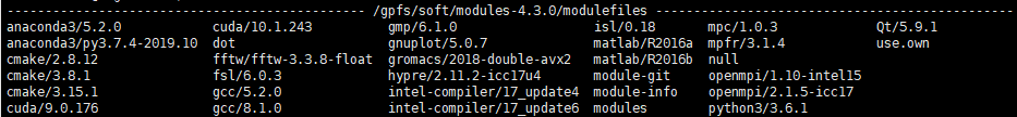
• module avail: Lists all available module files in the current module path.

[1907160330@login02 ~]$ module avail

• module load MODULEFILE: Load a module file/class.

[1907160330@login02 ~]$ module load matlab/R2016a

• module list: Display loaded modules.

[1907160330@login02 ~]$ module list
Currently Loaded Modulefiles:
 1) matlab/R2016a  

• module unload MODULEFILE: Unload a module file/class.

[1907160330@login02 ~]$ module unload matlab/R2016a
[1907160330@login02 ~]$ module list
No Modulefiles Currently Loaded.

• module switch MODULEFILE-A MODULEFILE-B: Switch modules.

This command unloads module A and loads module B.

[1907160330@login02 ~]$ module load matlab/R2016a
[1907160330@login02 ~]$ module list
Currently Loaded Modulefiles:
 1) matlab/R2016a  
[1907160330@login02 ~]$ module switch matlab/R2016a cmake/3.8.1
[1907160330@login02 ~]$ module list
Currently Loaded Modulefiles:
 1) cmake/3.8.1  
[1907160330@login02 ~]$ 

Custom MODULEFILE

When the administrator-configured MODULEs do not include the environment you need, regular users can create their own MODULEFILE files.

1. Go to the user's home directory and use the mkdir command to create a folder named privatemodules.

[1907160330@login02 ~]$ mkdir privatemodules
[1907160330@login02 ~]$ ls
3.6.1  ai_datastore  matlab-0  matlab_crash_dump.1099-1  privatemodules  soft

2. Enter the privatemodules folder and create a variable. Here we use ffmpeg as an example.

[1907160330@login02 privatemodules]$ mkdir ffmpeg
[1907160330@login02 privatemodules]$ cd ffmpeg
[1907160330@login02 ffmpeg]$ vim 4.3.1

This will open the vim editor. Enter or paste the following script (in English mode, press i to start editing):

#%Module1.0
proc ModulesHelp { } {
        puts stderr "\t FFmpeg  \n"
}
module-whatis "\t For more information, $module help ffmpeg \n"
conflict modulefile
prepend-path PATH /gpfs/users_home/1907160330/soft/ffmpeg

After editing, press Esc to exit edit mode, then type :wq! to save and exit.

3. Use cd ~ to return to the user's home directory and modify the current user's environment variable file .bashrc to add our self-built directory to module.

[1907160330@login02 ffmpeg]$ cd ~
[1907160330@login02 ~]$ vim .bashrc 

In English mode, press i to insert: export MODULEPATH=/gpfs/users_home/xxx/privatemodules:$MODULEPATH (where xxx is your username)

# .bashrc
# Source global definitions
if [ -f /etc/bashrc ]; then
        . /etc/bashrc
fi
# Uncomment the following line if you don't like systemctl's auto-paging feature:
# export SYSTEMD_PAGER=
export MODULEPATH=/gpfs/users_home/1907160330/privatemodules:$MODULEPATH
# User specific aliases and functions

After editing, press Esc to exit edit mode, then type :wq! to save and exit.

4. Use the source command to make your configuration file take effect.

[1907160330@login02 ~]$ source .bashrc
-bash: PROMPT_COMMAND: readonly variable

5. Use module av command to view, and you will see the MODULEFILE we added ourselves.

[1907160330@login02 ~]$ module avail
---------- /gpfs/users_home/1907160330/privatemodules ----------
ffmpeg/4.3.1  python3/3.7.1  

Note that Markdown does not support some specific HTML attributes, such as the id attribute (e.g., <a id="MODULEFILE_306"></a>). Therefore, these elements have been omitted in the Markdown version. Additionally, Markdown does not support HTML entities within <code> tags (such as ：), which have been converted to their corresponding characters (such as :). Images and code blocks have been formatted according to Markdown syntax.